American Journal of Operations Research
Vol. 2 No. 1 (2012) , Article ID: 17826 , 14 pages DOI:10.4236/ajor.2012.21003
Some Remarks on Application of Sandwich Methods in the Minimum Cost Flow Problem
1Institute of Mathematics, University of Silesia, Katowice, Poland
2Faculty of Mathematics and Natural Sciences, Cardinal Stefan Wyszyński University, Warsaw, Poland
Email: marta.kostrzewska83@gmail.com, leslawsocha@poczta.onet.pl
Received November 27, 2011; revised December 25, 2011; accepted January 12, 2012
Keywords: Bicriteria Network Cost Flow Problem; Sandwich Algorithms; Efficient Frontier; Stochastic Costs
ABSTRACT
In this paper, two new sandwich algorithms for the convex curve approximation are introduced. The proofs of the linear convergence property of the first method and the quadratic convergence property of the second method are given. The methods are applied to approximate the efficient frontier of the stochastic minimum cost flow problem with the moment bicriterion. Two numerical examples including the comparison of the proposed algorithms with two other literature derivative free methods are given.
1. Introduction
The network cost flow problems which describe a lot of real-life problems have been studied recently in many Operation Research papers. One of the basic problems in this field are the bicriteria optimization problems. Although there exist exact computation methods for finding the analytic solution sets of bicriteria linear and quadratic cost flow problems (see e.g. [1,2]), Ruhe [3] and Zadeh [4] have shown that the determination of these sets may be very perplexing, because there exists the possibility of the exponential number of extreme nondominated objecttive vectors on the efficient frontier of the considered problems. The fact that efficient frontiers of bicriteria linear and quadratic cost flow problems are the convex curves in  allows to apply the sandwich methods for a convex curve approximation in this field of optimization (see e.g. [5-8]). However, in some of these algorithms the derivative information is required. A derivative free method was introduced first by Yang and Goh in [8], who applied it to bicriteria quadratic minimum cost flow problems. The efficient frontiers of these problems are approximated by two piecewise linear functions called further approximation bounds, which construction requires solving of a number of one dimensional minimum cost flow problems. Unfortunately, the method introduced by Yang and Goh works under the assumption that the change of the direction of the tangents of the approximated function is less than or equal to
 . AlsoSiem et al. in [7] proposed an algorithm based only on the function value evaluation, with the interval bisection partition rule and two new iterative strategies for the determination of the new input data point in each iteration. Authors gave the proof of linear convergence of their algorithm.
In this paper we consider the generalized bicriteria minimum cost flow problem. We are interested in minimizing two cost functions, which satisfy some additional assumptions. Two sandwich methods for the approximation of the efficient frontier of this problem are presented. In the first method, based on the algorithm proposed by Siem et al. [7], new points on the efficient frontier are computed according to the chord rule or the maximum error rule by solving proper convex network problems. In the second method, we modify the lower approximation function discussed in [8], what decreases the Hausdorff distance between upper and lower bounds. We give the proofs of the linear convergence property of the first method called the Simple Triangle Algorithm and the quadratic convergence property of the second method called the Trapezium Algorithm.
The paper is organized as follows. In Section 2, we state a nonlinear bicriteria optimization problem that can be treated as a generalized minimum cost flow problem. In Section 3, two new sandwich methods of approximation of the efficient frontier of the stated problem are presented and in Subsection 3.5 the corresponding algorithms are presented. In Section 4, we discuss the convergence of these algorithms. Section 5 includes the information how to use the methodology from Section 2 in the case of the stochastic minimum cost flow problem with the moment bicriterion. To illustrate discussed methods in comparison with the algorithms presented in [7] and [8] two numerical examples are given. Finally, Section 6 contains the conclusions and future research direction. Proofs of lemmas and Theorem 2 are given in Appendix.
2. Problem Statement
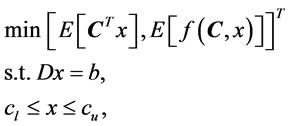
Let G be the directed network with n nodes and m arcs. Let . We consider the generalized minimum cost flow problem (GMCFP) defined as follows
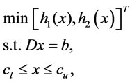 (1)
(1)
where  is the node-arc incidence matrix,
  is the net outflow of the nodes, vectors
  are the lower and upper capacity bounds for the flow
  and
and  are the cost functions such that
  is a continuous and convex function and
 where
where  and
and  is a continuous, concave and strictly increasing function. Let
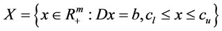
be the feasible set of problem (1).
According to the concept of Pareto optimality we consider the relations ≤ and < in  defined as follows
 and
and 
 and
and 
Using these definitions in the field of the bicriteria programming, a feasible solution  is called the efficient solution of problem (1) if there does not exist a feasible solution
  such that
 (2)
(2)
The set of all efficient solutions and the image of this set under the objective functions are called the efficient set and the efficient frontier, respectively.
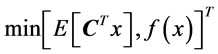
Note that the efficient set  of problem (1) is the same as the efficient set of following problem
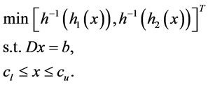 (3)
(3)
Moreover, from the fact that  for all
  and that the function
  is a convex one it follows the next lemma.
Lemma 1
Efficient frontier of problem (3) is a convex curve in .
.
Proof: See Appendix.
3. The New Sandwich Methods
In this section, we introduce two new sandwich methods for the approximation of the efficient frontier of problem (3).
3.1. Initial Set of Points
Let  and
and  and suppose that
 (4)
(4)
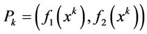
for all  are r given points on the efficient frontier of problem (1) such that
  and
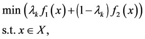
and  are the lexicographical minimum for the first and the second criterion, respectively. Although we need only three given points on the efficient frontier to start the first method called the Simple Triangle Method (STM) and two points to start the second method called the Trapezium Method (TM), the described methodologies work for any number r of initial points, which may be obtained by solving scalarization problems corresponding to problem (3), i.e.
 (5)
(5)
where  for all
 .
.
Another possibility is to find lexicographical minima of problem (3) and then to solve  convex programing problems with additional equality constraints
 (6)
(6)
where . This method gives r points on the efficient frontier with the following property
 (7)
(7)
for all .
.
3.2. Upper Bound
Suppose that the initial set  of points on the efficient frontier is given and that the points are ordered according to the first criterion
  for all
 .
.
The upper approximation function  of the frontier on the subinterval
  called the upper bound is defined as the straight line through the points
  and
and , that is
 (8)
(8)
for 
3.3. Lower Bounds
In the algorithms proposed at the end of this section we will use two different definitions of the lower approximation functions called the lower bounds.
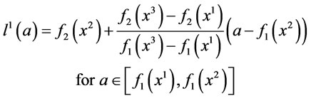
Definition 1
According to [7] the straight lines defined by the points  and
and  and the points
  and
and  approximate the frontier from below so the lower bound
  on the interval
  may be constructed in the following form
 (9)
(9)
where  and
and  is the point of intersecttion of two linear functions
  and
and .
.
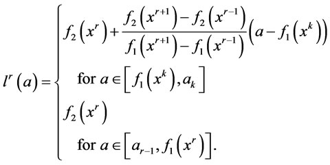
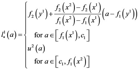
Moreover, we define the lower approximation bound  on the most left and the most right interval as follows
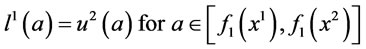 (10)
(10)
and
 (11)
(11)
where  is the point of intersection of function
  and the constant function
 .
.
If we compute new points on the efficient frontier due to the chord rule (see next section), then definition (9) may be modified, see Rote [9], in the following way
 (12)
(12)
where  and
and  is the point of intersection of corresponding two linear functions. Note that the lower bound is constructed by the tangents to
  and
and 
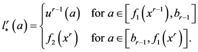
Moreover, the lower approximation bound  on the most left and the most right interval are redefined as follows
 (13)
(13)
and
 (14)
(14)
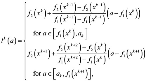
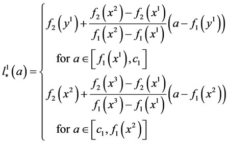
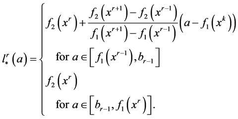
Definition 2
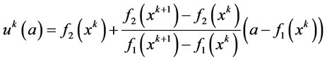
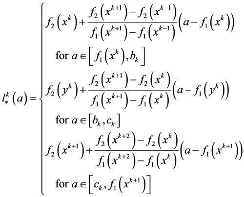
The simple modification of the definition presented in [8] leads to the following form of lower approximation bound  on the interval
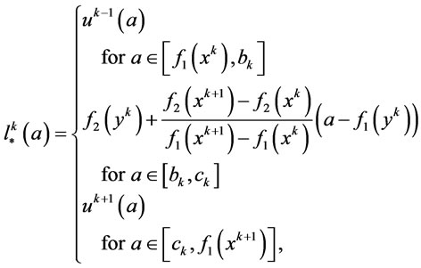 (15)
(15)
where , constants
  and
and  are the points of intersection of corresponding linear functions and
  is the solution of the following convex network problem (the chord rule problem)
 (16)
(16)
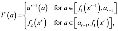
Similar to the previous case, we define the lower approximation bound on the most left and the most right interval as follows
 (17)
(17)
and
 (18)
(18)
Moreover, these definitions may be modified like in (12) using the tangents in points  in the following form
 (19)
(19)
and
 (20)
(20)
and
 (21)
(21)
If the approximation bounds  and
and  or
or  are constructed for each
 , then we define the upper approximation function
  of the efficient frontier of problem (3) in the following way
 (22)
(22)
and the lower approximation function due to equality
 (23)
(23)
or
 (24)
(24)
for all .
.
We note that after a small modification of the definition of the lower approximation function in the most right interval, any convex function may be approximated by the lower and upper bounds defined in this subsection.
3.4. Error Analysis
Suppose that the approximation bounds have been built and let , where
  denotes the approximation error on the interval
 . We consider three different error measures called the Maximum error measure (Maximum vertical error measure) (
 ), the Hausdorff distance measure (
 ) and the Uncertainty area measure (
 ) (see [7])
 (25)
(25)
 (26)
(26)
where
and
 (27)
(27)
If a measure  (one of
 ,
,  ,
, ) does not satisfy a desired accuracy, we choose
  for which
  and we determine the new point
 on the efficient frontier of problem (3) such that
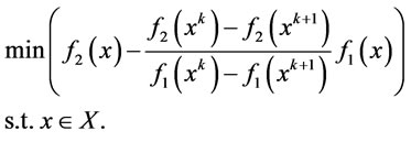
 . New points on the efficient frontier may be computed according to the chord rule or the maximum error rule, that is by solving the optimization problem (16) or the following problem (the maximum error rule problem)
 (28)
(28)
where  is the point of intersection of linear functions
  and
and  Note that if we construct the lower bound due to definition (15), then the chord rule problem (16) has been already solved.
After the determination of the new point, we rebuild the set P of given points on efficient frontier due to following equality
 (29)
(29)
then we construct new upper and lower bounds and repeat the procedure until we obtain an error  smaller than the prescribed accuracy.
The next lemma describes the relation between the approximation bounds of the efficient frontiers of problems (1) and (3).
Lemma 2
Let  and
and  be the lower and upper approximation bounds of the efficient frontier of problem (3) built due to the definitions (8) and (9) or (8) and (15), then
  and
and  are the lower and upper approximation bounds of the efficient frontier of problem (1).
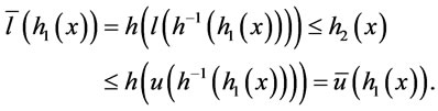
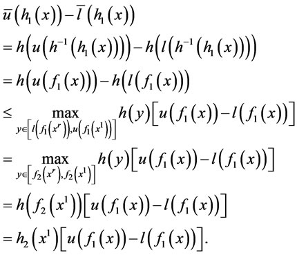
Moreover, the following inequality is satisfied
 (30)
(30)
for all the efficient solutions  and
and 
Proof: See Appendix.
From Lemma 2 follows that in order to obtain the Maximum error between upper and lower approximation bounds  and
and  of problem (1) smaller than or equal to the accuracy parameter
 , we need to build the approximation bounds
  and
and  of problem (3) for which the Maximum error is smaller than or equal to
  .
.
3.5. Algorithms
We present two algorithms described in this section.
3.5.1. The Simple Triangle Algorithm (STA)
Input: Introduce an accuracy parameter  and an initial set of points on the efficient frontier
 .
.
Step 1. Calculate lower and upper bounds ,
,  and error
 . Check if
 , then go to Step 2, otherwise stop.
Step 2. Choose interval  for which the maximum error is achieved. Solve the quadratic problem (16) or (28) to obtain the new point
 . Update set P, lower and upper bounds
 ,
,  and error
 . Go to Step 3.
Step 3. Check if , then go to Step 2, otherwise stop.
3.5.2. The Trapezium Algorithm (TA)
Input: Introduce an accuracy parameter  and an initial set of points on the efficient frontier
 .
.
Step 1. Solve problem (16) and calculate lower and upper bounds ,
,  and error
 . Check if
 , then go to Step 2, otherwise stop.
Step 2. Choose interval  for which the maximum error is achieved. The new point
  . Update set P, solve problem (13), calculate lower and upper bounds
 ,
,  and error
 . Go to Step 3.
Step 3. Check if , then go to Step 2, otherwise stop.
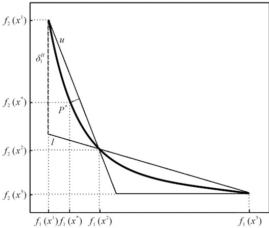
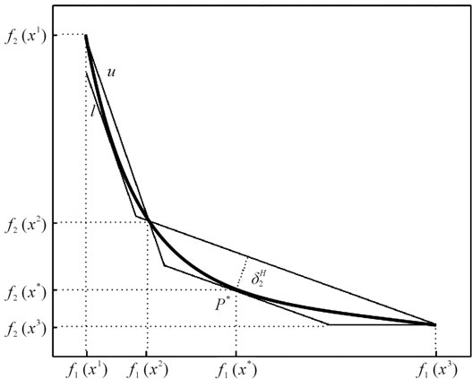
The geometric illustration of STA and TA is given in Figure 1 and Figure 2, respectively. In Figure 1(a), there is an illustration of an efficient frontier and the corresponding lower and upper bounds determined by three initial points
 (a)
(a)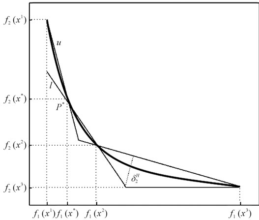 (b)
(b)
Figure 1. Lower and upper bounds built due to STA with the chord rule.

Here one can observe that in the interval  the Hausdorff measure
  is the greatest. It means that we have to introduce a new point
  into the efficient frontier and determine new corresponding lower and upper bounds, what is illustrated in Figure 1(b). Similar considerations are illustrated in Figures 2(a) and 2(b).
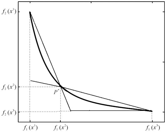
In Figure 3 and Figure 4 we see the illustration of STA and TA which lower bounds built due to definitions (9), (12) and (15), (19), respectively.
In Section 4 we study the convergence of described algorithms.
4. Convergence of the Algorithms
In this section we present the convergence results of presented algorithms based on proofs given in Rote [9]
 (a)
(a)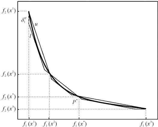 (b)
(b)
Figure 2. Lower and upper bounds built due to TA.
 (a)
(a)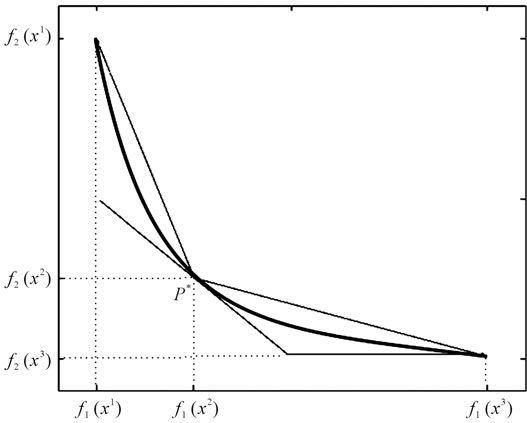 (b)
(b)
Figure 3. Lower bounds in STA built due to definitions (9) and (12) presented in (a) and (b), respectively.
and Yang and Goh [8]. First, we formulate two following remarks, which show the relation between the considered error measures.
Remark 1
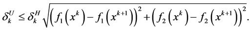
Suppose that the lower and upper approximation bounds on the interval  have been build according to the definitions (8) and (9) or (15), then we have
 (31)
(31)
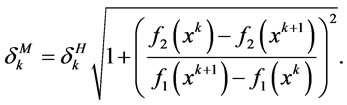
Moreover,
 (32)
(32)
See Figure 5.
 (a)
(a)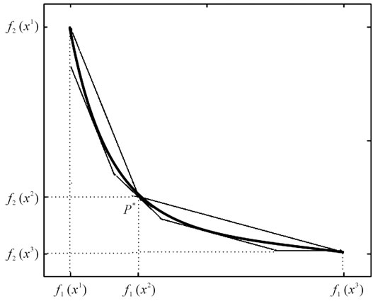 (b)
(b)
Figure 4. Lower bounds in TA built due to definitions (15) and (19) presented in (a) and (b), respectively.
Remark 2
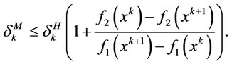
Suppose that the lower and upper approximation bounds on the interval  have been build according to the definitions (8) and (9) or (15), then we have
 (33)
(33)
Now, we suppose that the efficient frontier of problem (3) is given as a convex function  and the one-sided derivatives
  and
and  have been evaluated.
The following theorem based on Remark 3 and Theorem 1 in [8], Theorem 2 in [9] and Remark 1 and Remark 2 shows the quadratic convergence property of TA.
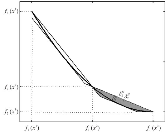
Figure 5. Illustration of error measures defined by (25)-(27).
Theorem 1
Let  and
and  and suppose that the point
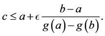
  was chosen to satisfy the following inequality
 (34)
(34)
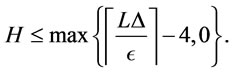
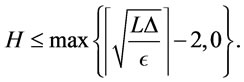
The number H of optimization problems (16) which have to be solved in order to obtain the Hausdorff distance between upper and lower bounds in TA smaller than or equal to  satisfies the following inequality
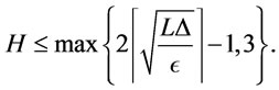 (35)
(35)
The third point  on the efficient frontier has to be chosen if we want to avoid the problems with the leftmost interval in which the Hausdorff distance between the approximation bounds is equal to the maximum error measure between them. The explanation how to determine a point with property (34) is given in the proof of Theorem 2.
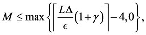
Corollary 1
Let 
 . The number M of optimization problems (16) which have to be solved in order to obtain the Maximum error between upper and lower bounds in TA smaller than or equal to
  satisfies the following inequality
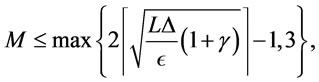 (36)
(36)
where 
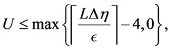
The number U of optimization problems (16) which have to be solved in order to obtain the Uncertainty area error between upper and lower bounds in TA smaller than or equal to  satisfies the following inequality
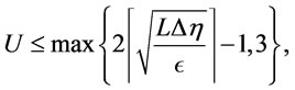 (37)
(37)
where 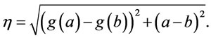
Yang and Goh [8] noticed that the right directional derivative  may be close to
 , that is why using the fact that the Hausdorff distance is invariant under rotation it is better to consider the efficient frontier rotated by
  with the modified directional derivatives
 and
and  and with
  as the projective distance of the segment between points
  and
and  onto the line
 .
.
Also for STA we may find the upper bound for the number of optimization problems (16) or (28) which have to be solved. First, let us formulate the following lemma.
Lemma 3
Suppose that the convex function  is approximated from below by two linear functions
  and
and  such that
 and
and  for some
  Let
Let  and
and  be the lines which intersect the points
 ,
,  and
and ,
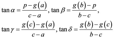
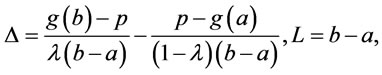
,  , respectively (see Figure 6). If we denote by
 ,
,  ,
,  ,
,  the slopes of lines
 ,
,  ,
,  ,
,  , respectively, then the following inequality is satisfied
 (38)
(38)
where 
 ,
, 
 and
and 
Proof: See Appendix.
Note that  and
and  are the differences of the slopes of lower approximation functions computed according to STA for interval
  and
and , respectively, and
  and
and  are the lengths of these intervals.
The next theorem based on Lemma 5, Theorem 2 from [9] and Lemma 3 establishes the linear convergence property of STA.
Theorem 2
Let ,
,  and
and  are three initial points which are necessary to start STA and suppose that
  was chosen to satisfy the following inequality
 (39)
(39)
Let  and let
 , then the number H of convex optimization problems ((16) or (28)), which have to be solved in order to make the Hausdorff distance between upper and lower bound in STA with the chord rule or the maximum error rule smaller than or equal to
  satisfies the following inequality
 (40)
(40)
Proof: See Appendix.
Corollary 2
Let ,
,  and
and  are three initial points that are necessary to start STA and suppose that
  was chosen to satisfy the inequality (39). Let
  and let
 . The number M of optimization problems (16) which have to be solved in order to obtain the Maximum error between upper and lower bounds in TA smaller than or equal to
  satisfies the following inequality
 (41)
(41)
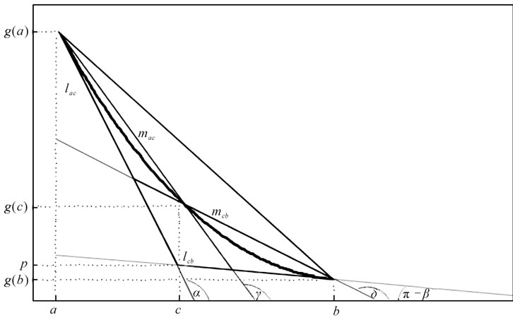
Figure 6. Illustration of functions and angels considered in Lemma 3.
where 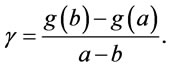 The number U of optimization problems (16) which have to be solved in order to obtain the Uncertainty area error between upper and lower bounds in TA smaller than or equal to
  satisfies the following inequality
 (42)
(42)
where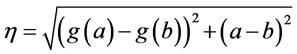 .
.
Remark 3
Note that this theorem is true for every convex function  such that the one-sided derivative
  has been evaluated. If we do not have the derivative information using TA with maximum error rule gives us the linear convergence property of this procedure.
The following theorem by Rote [9] establishes the quadratic convergence property of STA with the modified lower bound as in (12).
Theorem 3
Let ,
,  and
and  are three initial points which are necessary to start STA and suppose that
  was chosen to satisfy the following inequality
 (43)
(43)
Let  and let
 , then the number H of convex optimization problems (16), which have to be solved in order to make the Hausdorff distance between upper and lower bound in STA and TA with the modified lower bounds and the chord rule smaller than or equal to
  satisfies the following inequality
 (44)
(44)
5. Examples
In this section we define the stochastic minimum cost flow problem with the moment bicriterion and present two numerical examples, which illustrate algorithm presented in Section 3. Similar to the classic bicriteria network cost flow problem, we consider the directed network G with n nodes and m arcs with the node-arc incidence matrix , the net outflow vector
  and the capacity bounds
  Suppose that the cost per unit of flow through the arc
  is described by the random variable
  and assume that each variable
  has positive expected value
  and let C be a random vector such that
  The stochastic minimum cost flow problem with the moment bicriterion (SMCFP) is defined as follows
 (45)
(45)
where 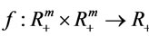 is the continuous function such that
 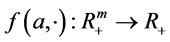 is convex for every
 .
.
Since  and
and  are linear and convex functions, respectively, then using Lemma 1 we find that the efficient frontier of problem (45) is a convex curve in
The following two examples include the comparison of the results obtained by STA, TA with Yang and Goh’s method [8] and the Siem et al.’s algorithm [7].
Example 1
We consider the simple stochastic minimum cost flow problem
 (46)
(46)
s.t.
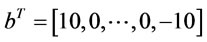
where 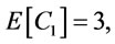

 and
and
 (47)
(47)
The vectors  and
and  are the lexicographical minima due to the first and the second criterion of problem (46) and
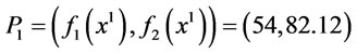
and
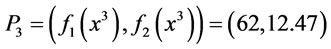
are corresponding to these vectors points on the efficient frontier. To avoid the problem with the leftmost interval we have taken  to be the third point of the efficient frontier necessary to start STA and TA.
The results’ comparison of subsequent calls of TA and Yang and Goh’s algorithm (YG) and the values of the Uncertainty area measure  after each step of TA with the lower bounds defined in (19) (TA1) are presented in Table 1. The results of STA, when new points are computed according to the maximum error rule in common with the Maximum error measure (STAM) and when new points are computed according to the chord rule in common with the Hausdorff measure with the lower bounds defined by the Equation (9) (STAH) and
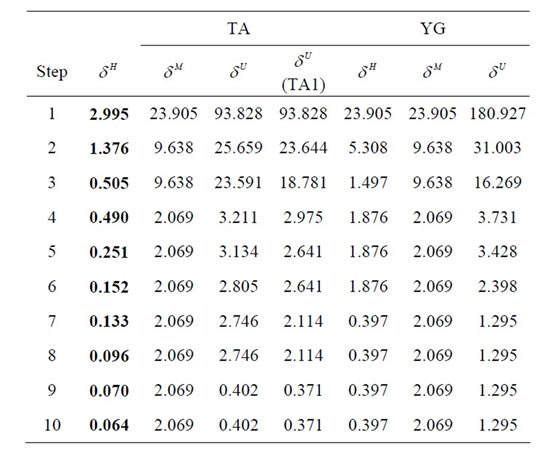
Table 1. The results of subsequent calls of TA and Yang and Goh’s method (YG) for the problem described in example 1.
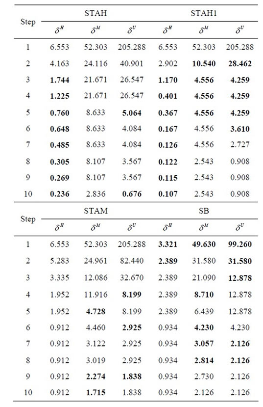
Table 2. The results of subsequent calls of STA with the chord rule (STAH, STAH1) and the maximum error rule (STAM) and Siem el al.’s method with interval bisection rule (SB) for the problem described in example 1.
(12) (STAH1) are summarized in Table 2. In the case of Yang and Goh’s method the errors are measured in the intervals set by the breakpoints of the upper bound. Table 2 includes also the results of the method described in [7], which uses the interval bisection method of the computing new points with the Maximum error measure. After each step of algorithm we present the maximum values of three error measures: the Maximum error, the Hausdorff distance and the Uncertainty area. As we can notice TA and TA1 performs better than other algorithms giving in each step the smallest values of the Hausdorff distance measure and the Uncertainty area measure. Moreover, from Table 2 we can conclude that STA with the chord rule and the Hausdorff distance gives smaller values of the Hausdorff measure in each step than to two other algorithms, which give comparable results.
Example 2
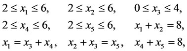
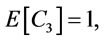
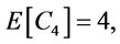
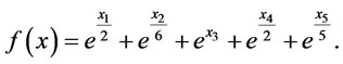
We consider the stochastic minimum cost flow problem in the network with 12 nodes and 17 arcs. We would like to minimize the mean value of the total cost of the flow through the network and the second moment of total cost, that is we solve the following problem
 (48)
(48)
where ,
,  ,
, 
and  and
and 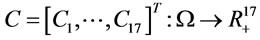
is the random cost vector such that  and
and  are mutually independent for all
  such that
 . We have chosen the values of
  from the interval
  and the values of the second moments
  from the interval
 . The points on the efficient frontier corresponding to the lexicographical minima of problem (48) and the second criterion are
  and
and  . In this example only TA and the Yang and Goh’s method are considered, since from Example 1. follows that these two algorithms work faster in comparison to STA and Siem et al.’s method. Table 3 includes the comparison of TA with the method presented in [8]. After each step of the considered methods we present the values of Hausdorff distance, Maximum error and Uncertainty area measure and a new evaluated point. As we can notice TA performs better in compareson to Yang and Goh’s algorithm giving in each step the smallest value of the Hausdorff distance between upper and lower approximation bounds.
6. Conclusions
Two sandwich algorithms (the Simple Triangle Algorithm
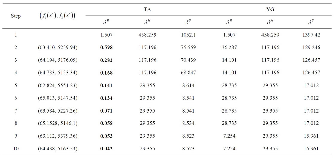
Table 3. The results of subsequent calls of TA and Yang and Goh’s method (YG) for the problem described in example 2.
and the Trapezium Algorithm) for the approximation of the efficient frontier of the generalized bicriteria minimum cost flow problem have been described. Both methods have been applied in the field of the stochastic minimum cost flow problem with the moment bicriterion.
The Simple Triangle Algorithm uses the lower bound proposed by Siem et al. in [7] with the maximum error rule or the chord rule, what causes faster decrease of the Maximum error measure and the Hausdorff distance measure and, as a result, reduces the number of steps of algorithm in comparison to the Siem et al.’s method. We have established the linear convergence property of this algorithm with both partition rules. If the lower bound in the Simple Triangle Algorithm is defined as in [9], according to the definition (12) and new points of the efficient frontier are computed due to the chord rule then we have the quadratic convergence property of the algorithm.
From the numerical examples follows that the Trapezium Algorithm performs better in comparison to all of the mentioned derivative free algorithms (Siem et al.’s method, Yang and Goh’s method) and gives in each step the smallest values of the Hausdorff distance measure between lower and upper bound. It also works faster than Rote’s triangle algorithm. Moreover, Trapezium Algorithm may be used for approximation of any convex function without the assumption that the change of the direction of the tangents of this function is less than or equal to , see [8]. The quadratic convergence property of the Trapezium Algorithm has been established.
For further research we are interested in the construction of a method for solving the stochastic minimum cost flow problem with the moment multicriterion.
REFERENCES
- A. Sedeno-Noda and C. Gonzalez-Martin, “The Biobjective Minimum Cost Flow Problem,” European Journal of Operational Research, Vol. 124, No. 3, 2000, pp. 591- 600. doi:10.1016/S0377-2217(99)00191-5
- X. Q. Yang and C. J. Goh, “Analytic Efficient Solution Set for Multi-Criteria Quadratic Programs,” European Journal of Operational Research, Vol. 92, No. 1, 1996, pp. 166-181. doi:10.1016/0377-2217(95)00040-2
- G. Ruhe, “Complexity Results for Multicriterial and Parametric Network Flows Using a Pathological Graph of Zadeh,” Zeitschrift für Operations Research, Vol. 32, No. 1, 1988, pp. 9-27. doi:10.1007/BF01920568
- N. Zadeh, “A Bad Network for the Simplex Method and Other Minimum Cost Flow Algorithms,” Mathematical Programming, Vol. 5, No. 1, 1973, pp. 255-266. doi:10.1007/BF01580132
- R. E. Burkard, H. W. Hamacher and G. Rote, “Sandwich Approximation of Univariate Convex Functions with an Applications to Separable Convex Programming,” Naval Research Logistics, Vol. 38, 1991, pp. 911-924.
- B. Fruhwirth, R. E. Burkard and G. Rote, “Approximation of Convex Curves with Application to the Bi-Criteria Minimum Cost Flow Problem,” European Journal of Operational Research, Vol. 42, No. 3, 1989, pp. 326-338. doi:10.1016/0377-2217(89)90443-8
- A. Y. D. Siem, D. den Hertog and A. L. Hoffmann, “A Method for Approximating Univariate Convex Functions Using Only Function Value Evaluations,” Center Discussion Paper, Vol. 67, 2007, pp. 1-26.
- X. Q. Yang and C. J. Goh, “A Method for Convex Curve Approximation,” European Journal of Operational Research, Vol. 97, No. 1, 1997, pp. 205-212. doi:10.1016/0377-2217(95)00368-1
- G. Rote, “The Convergence Rate of the Sandwich Algorithm for Approximating Convex Functions,” Computing, Vol. 48, No. 3-4, 1992, pp. 337-361. doi:10.1007/BF02238642
Appendix
We present the proofs of Lemma 1, Lemma 2, Lemma 3 and Theorem 2.
Proof of Lemma 1
Let ,
,  and let
 for
for  be two given points on the efficient frontier of problem (3) and let
 .
.
If  then for all b such that
 the point
  lies also on the efficient frontier of problem (3).
Suppose now that . Note that for
 (49)
(49)
 (50)
(50)
and
 (51)
(51)
we have , what yields
 (52)
(52)
Due to the convexity of the function  we have
 (53)
(53)
what proves the convexity of the efficient frontier of problem (3). 
Proof of Lemma 2
Let , then we have
 (54)
(54)
what is equivalent to the following inequality
 (55)
(55)
and from the fact that  is increasing we have
 (56)
(56)
Moreover,
 (57)
(57)

Proof of Lemma 3
Let , where
  and let
  Without loss of generality we may assume that
 , then we have
 .
.
From the equalities
 (58)
(58)
follows
 (59)
(59)
 (60)
(60)
 (61)
(61)
Now, it is easy to show that inequality (38) is equivalent to
 (62)
(62)
Using the fact that  we complete the proof.
Proof of Theorem 2
Suppose that we have found point  with property (39). It is possible to find such a point as a solution of a convex programing problem with one additional constraint similar to problem (6). From condition (39) follows that
  and
and .
.
Now, if we consider the interval , then we have
  and
and
Similar to [9] we prove the theorem by induction on number .
.
The induction basis,  , is equivalent to Lemma 1 from [5], which also holds for lower approximation function built according to definition (9).
Suppose that . If after one step of STA
 , then we have had only one additional evaluation and the thesis is true.
In the other case, let  be the new computed point and let
  and
and  Let
Let  and
and  denote the slope differences of the linear functions building the lower bounds in the interval
  and
and , respectively. We can assume without lost of generality that the error
  exceeds
  in the right subinterval. Lemma 5 and Lemma 1 from [9] used for the lower approximation bounds built due to definition (9) give the following inequalities
 (63)
(63)
and
 (64)
(64)
Lemma 3 and inequality (63) gives
 (65)
(65)
Similarly, Lemma 3 and inequality (64) gives
 (66)
(66)
From (65) and (66) we have
 (67)
(67)
Now the induction hypothesis can be applied for  and
and  If
If , then the theorem’s thesis follows directly.
Otherwise, from Lemma 3 we have
 (68)
(68)
what ends the proof. 