Intelligent Information Management
Vol.2 No.11(2010), Article ID:3234,6 pages DOI:10.4236/iim.2010.211072
Record Values from the Inverse Weibull Lifetime Model: Different Methods of Estimation
Department of Statistics and Operations Research, College of Science, King Saud University, Riyadh, Saudi Arabia
E-mail: ksultan@ksu.edu.sa
Received September 21, 2010; revised October 13, 2010; accepted November 15, 2010
Keywords: Scale Parameter, Location Parameter, Best Linear Unbiased Estimates (BLUEs), Maximum Likelihood Estimates, Relative Efficiency and Monte Carlo Simulations
Abstract
In this paper, we use the lower record values from the inverse Weibull distribution (IWD) to develop and discuss different methods of estimation in two different cases, 1) when the shape parameter is known and 2) when both of the shape and scale parameters are unknown. First, we derive the best linear unbiased estimate (BLUE) of the scale parameter of the IWD. To compare the different methods of estimation, we present the results of Sultan (2007) for calculating the best linear unbiased estimates (BLUEs) of the location and scale parameters of IWD. Second, we derive the maximum likelihood estimates (MLEs) of the location and scale parameters. Further, we discuss some properties of the MLEs of the location and scale parameters. To compare the different estimates we calculate the relative efficiency between the obtained estimates. Finally, we propose some numerical illustrations by using Monte Carlo simulations and apply the findings of the paper to some simulated data.
1. Introduction
Record values arise naturally in many real life applications involving data relating to weather, sport, economics and life testing studies. Many authors have studied record values and the associated statistics; see, for example, [1-7]. Reference [8] has established some recurrence relations for the moments of record values from the Gumbel distribution. Similar work has been carried out by [9,10] for the generalized extreme value and exponential distributions, respectively. Reference [11] have also discussed some inferential methods based on record values from Gumbel distribution. [12,13] have discussed inferential techniques based on Weibull and generalized Pareto distributions, respectively. Reference [14] have compared different estimates based on record values from Weibull distribution. Reference [15] has considered different loss functions to develop the Bayesian estimates of the parameters of the IWD.
Let  be the first
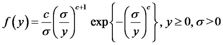
  lower record values from the IWD with density function
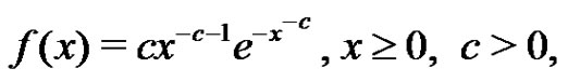 (1.1)
(1.1)
and cumulative distribution function ( )
)
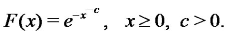 (1.2)
(1.2)
The scale form of the IWD has its density function given by
 (1.3)
(1.3)
while the location-scale IWD has its density function given by
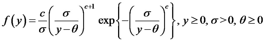 (1.4)
(1.4)
Reference [16] calls the IWD as the complementary Weibull distribution, while [17] call it the reciprocal Weibull distribution. Reference [18] have discussed some useful measures for the IWD.
The IWD plays an important role in many applications, including the dynamic components of diesel engines and several data set such as the times to breakdown of an insulating fluid subject to the action of a constant tension. [19] provide an interpretation of the IWD in the context of the load-strength relationship for a component. Reference [20] has fitted the IWD to the flood data. For more details on the IWD, see for example, [21].
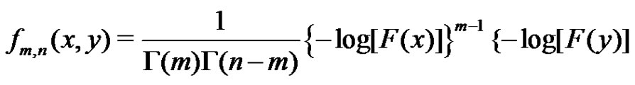
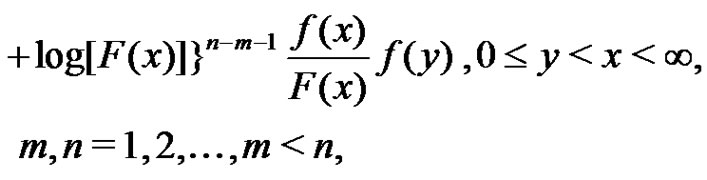
The joint density function of the first  lower record values
  is given by [5]
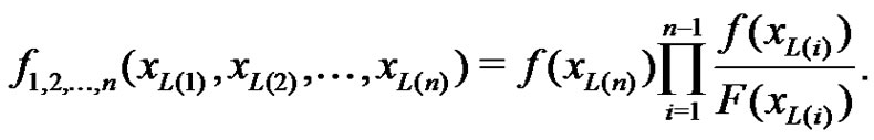 (1.5)
(1.5)
From (1.5), the  of
of  can be obtained as
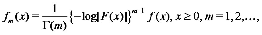
(1.6)
where  and
and  are given in (1.1) and (1.2), respectively.
The the joint  of
of  and
and  is given by
 (1.7)
(1.7)
where  and
and  are given in (1.1) and (1.2), respectively.
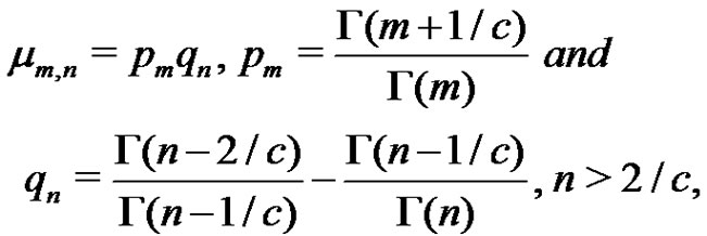
The single and product moments of record values are (see [22])
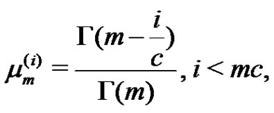 (1.8)
(1.8)
and
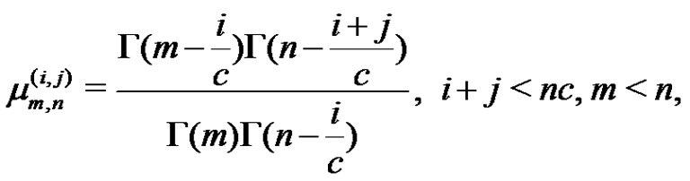 (1.9)
(1.9)
where  is the gamma function.
In the following section, we derive the exact form of the BLUE scale parameter and present the BLUEs of the location-scale case of IWD. Next in Section 3, we derive the maximum likelihood estimates of the parameters of IWD. Finally, in Section 4 we discuss the relative efficiency of the obtained estimates.
2. The BLUEs
In this section, we derive the BLUE of the scale parameter and present the BLUEs of the location and scale parameters of the IWD.
2.1. The Scale Case
Let  denote the first
  lower record from the distribution in (1.3), and let
  be the corresponding record values from the IWD in (1.1). Assume
and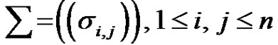 . Then, the BLUE of the scale parameter
  is given by
 (2.1)
(2.1)
and its variance is given by
 (2.2)
(2.2)
for details, refer to [23,6]. Since the double moment  can be written as
 (2.3)
(2.3)
then the covariance matrix  can be inverted analytically. Then
  element
  of
of  can be derived as
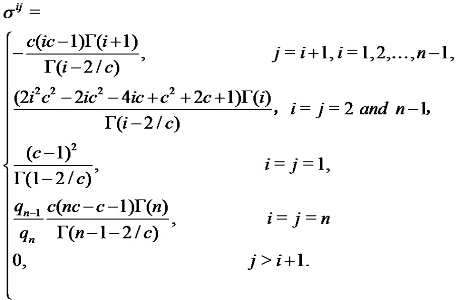
(2.4)
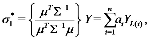
From (1.8), (2.1) and (2.4), we have the BLUE of the scale parameter  as
as
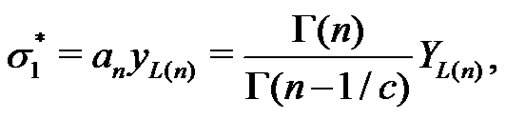 (2.5)
(2.5)
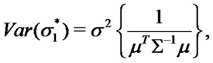
with variance is given by
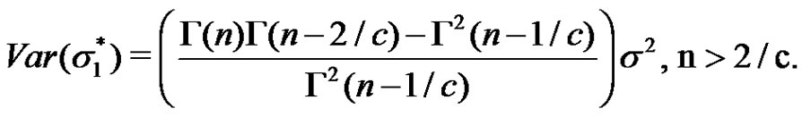 (2.6)
(2.6)
It is clear from (2.5) that  is an unbiased estimate of
 .
.
Table 1 below shows the coefficients  of the BLUE of
  when
when  to
to  and
and .
.
The BLUE of  given in (2.5), can be used to construct
  confidence interval for
  through the formula
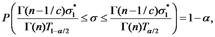 (2.7)
(2.7)
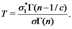
where  and
and  are the lower and upper percentage points of the pivotal quantity
The cdf of  is obtained to be
 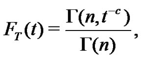 where
where  is the incomplete gamma function.
Example
Five lower record values are simulated from IWD with  and
and  as follows: 3.07586, .90607, 68454, .62296, .62283, by using the coefficients of the BLUE of the scale parameter given in Table 1, we have
  and the standard error of this estimate is
 Now, we calculate the lower and upper
 percentage points of of
  to be
to be
 and
and .
.
Then  confidence interval for
  can be calculated from (2.7) to be
 .
.
2.2. The location-Scale Case
Reference [15] has used the single and product moments of the record values from IWD. Then, he has used these moments to calculate the coefficients of BLUEs and the variances for records of size 4,5,6 and 7 and  by using the forms (see [23]).
 (2.8)
(2.8)
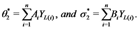
Table 2 represents the coefficients of the BLUEs  and
and  for records of sizes 4, 5, 6, 7 and the shape parameter
 . while Table 3 represents the variances and covariances of the BLUEs in this case.
Reference [24] has used the coefficients of BLUEs in Table 2 to construct different confidence intervals for the location and scale parameters of IWD based on Edgeworth approximation and compare them with those based on Monte Calro simulation.
3. The MLEs
In this section, we discuss the maximum likelihood estimates of the parameters of IWD when the available data are lower record values. We consider two different cases: 1) the scale-parameter case and 2) the locationscale parameter case.
3.1. The Scale-Parameter Case
Let 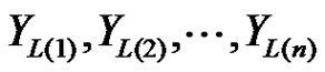 represents the first
  lower record values from the scale-parameter IWD in (1.3), then the log likelihood function is given by
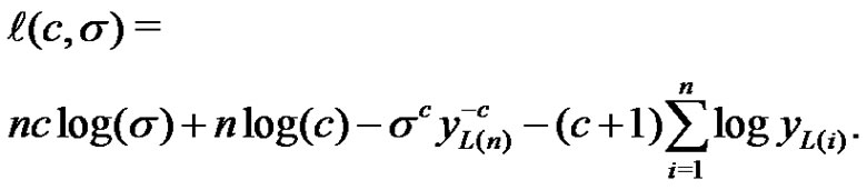 (3.1)
(3.1)
Now, we discuss two cases. They are:
1) When  unknown and
  known: the maximum likelihood estimate of
  can be obtained from (3.1) as
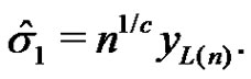 (3.2)
(3.2)
2) When both of  and
and  are unknown: the maximum likelihood estimates of
  and
and  can be obtained from (3.2) by solving the following two equations as
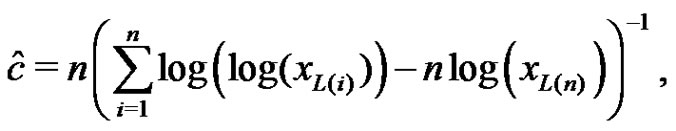 (3.3)
(3.3)
and
 (3.4)
(3.4)
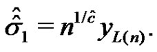
From (3.2), we see that
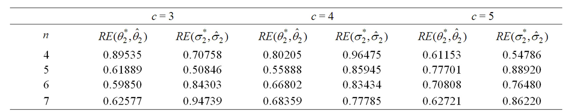
Table 1. The coefficients of the BLUE of the scale parameter and the variance when .
.
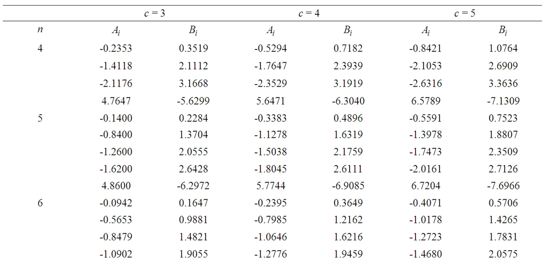
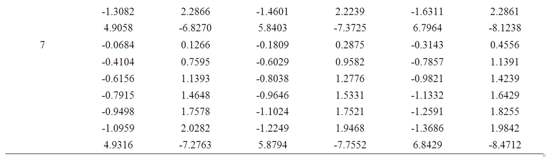
Table 2. The Coefficients of the BLUEs.
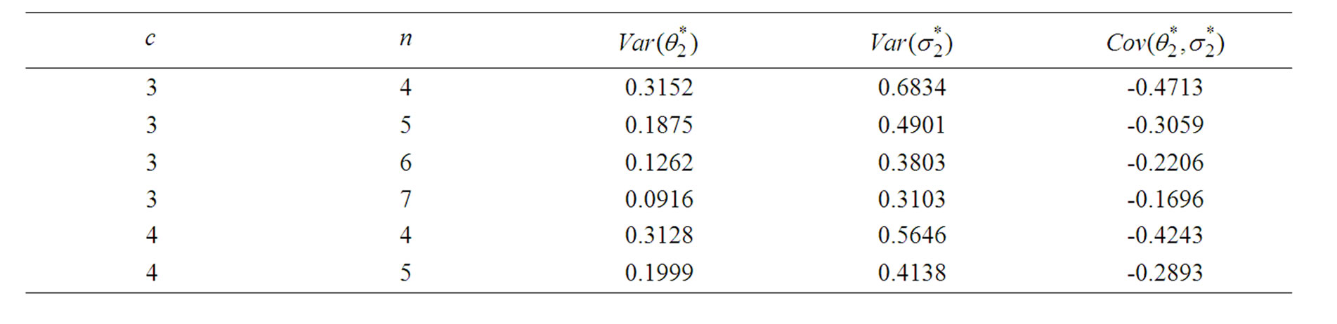
Table 3. The variances and covariances of the BLUEs when .
.
 (3.5)
(3.5)
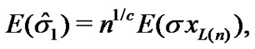
which upon using (1.8) gives
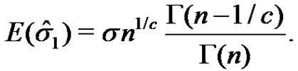 (3.6)
(3.6)
This shows that
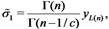 (3.7)
(3.7)
is an unbiased estimate for  in this case.
The variance of  is calculated to be
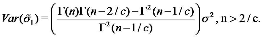 (3.8)
(3.8)
Lemma 1
The MLE of  given in (3.2) is asymptotically unbiased and its variance converges to zero as
 .
.
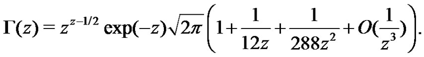
Proof The proof can be easily done by using the expansion of gamma function see [24]
3.2 The Location-Scale Case
When  represents the first n lower record values from the location-scale parameter IWD given in (1.4), then the log likelihood function is given by
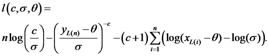
(3.9)
Now, we discuss two cases. They are:
1) When  is known: the maximum likelihood estimates of
  and
and  can be obtained by solving the following two equations
 (3.10)
 (3.11)
Table 4 below displays the bias and the estimated variance of the MLEs of the location and scale parameters in this case.
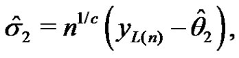
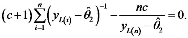
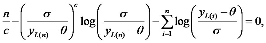
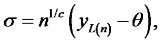
2) When  is unknown: the maximum likelihood estimates of
 ,
,  and
and  can be obtained from (3.9) by solving the following three equations as
(3.12)
 (3.13)
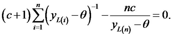 (3.14)
4 Relative Efficiency
To compare between the BLUEs and the MLEs obtained in Sections 2 and 3, we calculate the relative efficiency in some cases as follows:
1) For the scale case we have 
2) For the location-scale case we have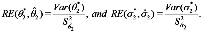
Table 5 given below show the relative efficiency be
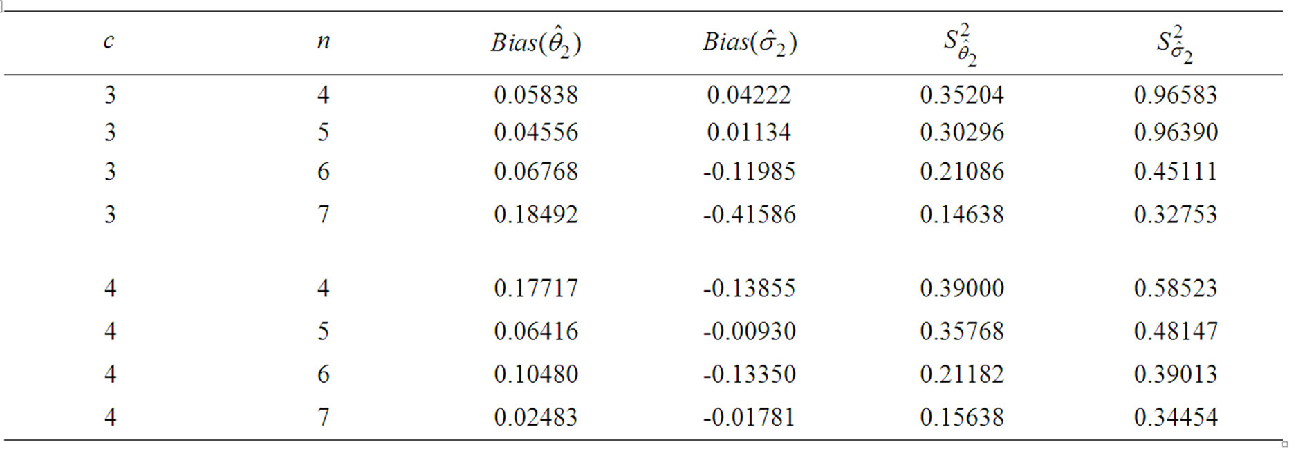
Table 4. The bias and estimated variance of the MLEs.
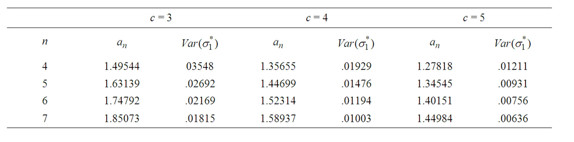
Table 5. The relative efficiency.
-tween the different estimates of the location and scale parameters. From Table 5, we see that, the BLUEs give more efficiency than the MLEs.
5. Acknowledgements
The author would like to thank the referees for their helpful comments, which improved the presentation of the paper. Also, the author would like to thank the Research Center, College of Science, King Saud University, for funding the project (Stat/2008/31).
6. References
[1] K. N. Chandler, “The Distribution and Frequency of Record Values,” Journal of the Royal Statistical Society Series B, Vol. 14, 1952, pp. 220-228.
[2] V. B. Nevzorov, “Records,” Theory of Probability and Its Applications, Vol. 32, 1988, pp. 201-228.
[3] H. N. Nagaraja, “Record Values and Related Statistics-A Review,” Communications in Statistics-Theory and Methods, Vol. 17, 1988, pp. 2223-2238.
[4] M. Ahsanullah, “Introduction to Record Values,” Ginn Press, Needham Heights, Massachusetts, 1988.
[5] M. Ahsanullah, “Record values, The Exponential Distribution: Theory, Methods and Applications,” In: N. Balakrishnan and A.P. Basu Eds., Gordon and Breach Publishers, Newark, New Jersey, 1995.
[6] B. C. Arnold, N. Balakrishnan and H. N. Nagaraja, “A First Course in Order Statistics,” John Wiley & Sons, New York, 1992.
[7] B. C. Arnold, N. Balakrishnan and H. N. Nagaraja, “Records,” John Wiley & Sons, New York, 1998.
[8] N. Balakrishnan, M. Ahsanullah and P. S. Chan, “Relations for Single and Product Moments of Record Values from Gumbel Distribution,” Statistics & Probability Letters, Vol. 15, No. 3, 1992, pp. 223-227.
[9] N. Balakrishnan, P. S. Chan and M. Ahsanullah, “Recurrence Relations for Moments of Record Values from Generalized Extreme Value Distribution,” Communications in Statistics-Theory and Methods, Vol. 22, No. 5, 1993, pp. 1471-1482.
[10] N. Balakrishnan and M. Ahsanullah, “Relations for Single and Product Moments of Record Values from Exponential Distribution,” Journal of Applied Statistical Science, Vol. 2, 1995, pp. 73-87.
[11] N. Balakrishnan, M. Ahsanullah, and P. S. Chan, “On the Logistic Record Values and Associated Inference,” Journal of Applied Statistics, Vol. 2, pp. 233-248.
[12] K. S. Sultan and N. Balakrishnan, “Higher Order Moments of Record Values from Rayleigh and Weibull Distributions and Edgeworth Approximate Inference,” Journal of Applied Statistical Science, Vol. 9, 1999, pp. 193-209.
[13] K. S. Sultan and M. E. Moshref, “Higher Order Moments of Record Values from Generalized Pareto Distribution and Associated Inference,” Metrika, Vol. 51, 2000, pp. 105- 116.
[14] A. A. Soliman, A. H. Abd Ellah and K. S. Sultan, “Comparison of Estimates Using Record Statistics from Weibull Model: Bayesian and Non-Bayesian Approaches,” Computational Statistics and Data Analysis, Vol. 51, No. 3, 2006, pp. 2065-2077.
[15] K. S. Sultan, “Higher Order Moments of Record Values from the Inverse Weibull Lifetime Model and Edgeworth Approximate Inference,” International Journal of Reliability and Applications, Vol. 8, No. 1, 2007, pp. 1-16.
[16] A. Drapella, “Complementary Weibull Distribution: Unknown or Just Forgotten,” Quality and Reliability Engineering International, Vol. 9, 1993, pp. 383-385.
[17] G. S. Mudholkar and G. D. Kollia, “Generalized Weibull family: A Structural Analysis,” Communications in Statistics-Theory and Methods, Vol. 23, 1994, pp. 1149- 1171.
[18] R. Jiag, D. N. P. Murthy and P. Ji, “Models Involving two Inverse Weibull Distributions,” Reliability Engineering and System Safety, Vol. 73, No. 1, 2001, pp. 73-81.
[19] R. Calabria and G. Pulcini, “On the Maximum Likelihood and Least-Squares Estimation in the Inverse Weibull Distributions,” Statistica Applicata, Vol. 2, No. 1, 1990, pp. 53-66.
[20] M. Maswadah, “Conditional Confidence Interval Estimation for the Inverse Weibull Distribution Based on Censored Generalized Order Statistics,” Journal of Statistical Computation Simulation, Vol. 73, No. 12, 2003, pp. 887- 898.
[21] D. N. P. Murthy, M. Xie and R. Jiang, “Weibull Models,” John Wiley & Sons, New York, 2004.
[22] E. M. Nigm and R. F. Khalil, “Record Values from Inverse Weibull Distribution and Associated Inference,” Bulletin of the Faculty of Science, 2006.
[23] N. Balakrishnan and A. C. Cohen, “Order Statistics and Inference: Estimation Methods,” Academic Press, San Diego, 1991.
[24] M. Abramowitz and I. A. Stegun, “Handbook of Mathematical Functions with Formulas, Graphs and Mathematical Tables,” Dover, New York, 1972.