Vol.2, No.10, 1130-1137 (2010) Natural Science
http://dx.doi.org/10.4236/ns.2010.210140
The Rich-Gini-Simpson quadratic index of biodiversity
Radu Cornel Guiasu1, Silviu Guiasu2
1Environmental and Health Studies Program, Department of Multidisciplinary Studies, Glendon College, York University, Toronto,
Canada; [e-mail];
2Department of Mathematics and Statistics, Faculty of Pure and Applied Sciences, York University, Toronto, Canada;
Received 6 August 2010; revised 10 September 2010; accepted 13 September 2010.
ABSTRACT
The Gini-Simpson quadratic index is a classic
measure of diversity, widely used by ecologists.
As shown recently, however, this index is not
suitable for the measurement of beta diversity
when the number of species is very large. The
objective of this paper is to introduce the Rich-
Gini-Simpson quadratic index which preserves
all the qualities of the classic Gini-Simpson in-
dex but behaves very well even when the num-
ber of species is very large. The additive parti-
tioning of species diversity using the Rich-Gini-
Simpson quadratic index and an application from
island biogeography are analyzed.
Keywords: Rich-Gini-Simpson Index of Species
Diversity; Additive Partitioning of Diversity; Island
Biogeography; Biodiversity
1. INTRODUCTION
Measuring the diversity of species in a habitat has
been an important area of interest in fields such as con-
servation biology, ecology, and biogeography for the last
several decades [1]. Let us assume that there are n
species and let:
1,=),,1,=(0,> i
i
ipnip 
 (1)
be the relative frequency distribution of these species in
the respective habitat. There are three classic measures
of diversity:
a) The number of species, or richness: n;
b) The Gini-Simpson quadratic index (abbreviated in
this paper as GS ):
,1=)(1= 2
i
i
ii
i
pppGS   (2)
introduced by Gini [2] and adapted for biological studies
by Simpson [3];
c) The Shannon entropy (abbreviated as
H
):
,ln=ii
i
ppH  
(3)
introduced by Shannon [4], as the discrete variant of the
continuous entropy defined by Boltzmann [5] in statisti-
cal mechanics. There is an extensive literature [1,6-17]
about the properties and applications of these measures
of diversity.
When the number of species n and the relative
abundance of species (1) are the only sources of infor-
mation available, many other measures of diversity have
been proposed. Recently, Jost [18,19] pleaded in favor of
the “true” measure of diversity, introduced by Hill [20]:
.=
)1/(1 r
r
i
i
rpN







(4)
For 0=r, we get: nN =
0. For 1=
r
, r N is not
defined because the denominator of the exponent,
r

1,
is equal to zero. However, the limit of r N when
r
tends to 1 is )(exp H. For 2=
r
we get )1/(1 GS

. In
fact, the natural logarithm of (4), i.e. r Nln , is just Ré-
nyi’s entropy [21]. There are no sound reasons to call (4)
a “true” measure of diversity. It is simply a unifying no-
tation, as mentioned in [20]. Besides, by performing ma-
thematical transformations on classic measures of diver-
sity, like taking the exponential of the Shannon entropy
or the reciprocal of the Gini-Simpson quadratic index,
for example, we obtain other measures that lose, how-
ever, some essential features of the original measures,
such as concavity, for instance. Concavity is an essential
property of any measure that can be used in an additive
partitioning of species diversity. Hoffmann and Hoff-
mann [22] are right when asking: “Is there a ‘true’ mea-
sure of diversity?” As noticed by Ricotta [23], there is a
“jungle of measures of diversity” in the current conser-
vation biology literature. Under the circumstances, per-
haps the best strategy is to remember Occam’s razor and,
trying to keep things simple, it may be easier to just go

R. C. Guiasu et al. / Natural Science 2 (2010) 1130-1137
113
1131
back to the classic measures of diversity mentioned be-
fore and see how they can be adjusted to address new
problems under new circumstances.
The species richness n is very simple but ignores the
abundance of species. Shannon’s entropy has excellent
properties but is difficult to estimate and maximizing it
subject to linear constraints, generally gives a solution
satisfying exponential equations which cannot be solved
analytically. On the other hand, the Gini-Simpson quad-
ratic index is simpler and generally seems to be pre-
ferred by ecologists. Jost [18,19,24], however, noticed a
troubling anomaly related to GS . Indeed, if this meas-
ure is used in the additive partitioning of species diver-
sity, the corresponding beta diversity approaches zero
when the number of species is very large. Thus, for two
habitats with no species in common, for instance, the
between-habitat diversity tends to zero when the number
of species in one of the habitats, or in both of them,
tends to infinity, instead of becoming larger as is obvi-
ously the case in actual fact.
The objective of this paper is to show that the anom-
aly just mentioned can be easily fixed. The product be-
tween the species richness a) and the measure of diver-
sity c), called here the Rich-Gini-Simpson quadratic in-
dex and abbreviated as RGS , preserves all the basic
properties of GS and behaves well when the number
of species is large. Therefore, RGS is suitable for use
in the additive partitioning of species diversity. Subse-
quently, the RGS index is applied to data on the avi-
faunal diversity on several tropical Indian Ocean islands,
using some of the numerical results obtained by Adler
[25], in order to show how the alpha, beta, and gamma
species diversities change when the usual equal weights
for the various habitats are replaced by the relative areas
and the relative elevations of the respective islands.
2. THE RICH-GINI-SIMPSON INDEX
If there are n species in a certain habitat and their
relative abundance is given by (1), the Rich-Gini-Simp-
son quadratic index is
).(1=)(1= 2
i
i
ii
i
pnppnRGS   (5)
The concavity of RGS and the maximum value of
RGS are analyzed in the Appendix. Thus, we have:
10  nRGS , the maximum corresponding to the
uniform distribution: npi1/= , ),1,=( ni . As
nRGSGS/= , the maximum value of GS is
nGS
p1/1=
max , corresponding to the uniform distri-
bution as well. The essential difference between these
two indexes is that GS is bounded by 1 and tends to 1
when the number of species n tends to infinity,
whereas RGS is not bounded and tends to infinity
when the number of species n tends to infinity. Shan-
non’s entropy, on the other hand, has the maximum
nH
pln=
max , which tends to infinity when the number
of species n tends to infinity, but it increases much
much more slowly than 1=
max nRGS
p.
Pleading against the use of the GS index, Jost [24]
gave the following example: “Suppose a continent has a
million equally-common species, and a meteor impact
kills 999,900 of the species, leaving 100 species un-
touched. Any biologist, if asked, would say that this me-
teor impact caused a large absolute and relative drop in
diversity. Yet GS only decreases from 0.999999 to
0.99, a drop of less than 1%”. Jost concluded that: “[The]
ecologists relying on GS will often misjudge the mag-
nitude of ecosystem changes. This same problem arises
when Shannon entropy is equated with diversity. In con-
trast, 
2
N drops by the intuitively appropriate
99.99%”. This example shows that there is indeed a
troubling anomaly in using GS when the number of
species is very large. But RGS has no such a drawback.
Indeed, if before the cataclysm there are 1,000,000=n
equally abundant species, then:
;13.8155105=ln=0.999999;=
1
1= nH
n
GS 
1000000,==)ln(exp=)(exp nnH
999999.=1=1000000,==
2nRGSnN
After the cataclysm, there are only 100=n equally
abundant species left. Thus:
6;4.60517018=0.99;=
1
1= H
n
GS 
100,==)ln(exp=)(exp nnH
99.=1=100,==
2nRGSnN
Therefore, GS indicates a decrease in diversity equal
to 0.999901%, which is obviously wrong,
H
indi-
cates a decrease in diversity equal to 7% 66.6666666,
which is not good enough, whereas RGS , )(exp H and
2
N give a decrease in diversity equal to 9% 99.9900999
and 0% 99.9900000, respectively, in agreement with
common sense. Let us note that, practically, RGS and
)(exp H have the same maximum value when the
number of species n is given, but the index )(expH
is not a concave function of the relative frequency dis-
tribution of species ),,(= 1n
ppp  and, consequently,
it is not suitable to be used in the additive partitioning of
species diversity, whereas the index RGS is.
3. THE ADDITIVE PARTITIONING OF
SPECIES DIVERSITY USING RGS
MacArthur [26] pointed out the need for a theory of
within-habitat and between-habitat species diversities.
Identify applicable sponsor/s here. (sponsors)

R. C. Guiasu et al. / Natural Science 2 (2010) 1130-1137
1132
He, together with Recher and Cody [27], proposed a
measure of the difference between the species diversities
of two habitats based on Shannon’s entropy and using
equal relative weights for habitats. This measure was
also used in the influential book “The theory of island
biogeography” by MacArthur and Wilson [28]. Rao [29],
without mentioning the paper [27], extended the measure
of the difference between the species diversities of two
habitats, based also on Shannon’s entropy but using ar-
bitrary weights assigned to the two habitats. Whittaker
[30,31] proposed linking diversity components between
ecological scales by multiplication so that the gamma
diversity, measuring the species diversity in a larger re-
gion consisting of several ecological communities taken
together, is the product of the alpha diversity, which
measures the mean species diversity in the local com-
munities taken separately, and the beta diversity, repre-
senting the variation and changes in mean species diver-
sity in a larger region which contains the local ecological
communities taken together, as a whole. The beta diver-
sity essentially measures the biogeographic changes in
species diversity among various locations within a larger
region. As such, the beta diversity can be important in
leading to the development of geographic strategies for
the conservation of species and habitats, as mentioned
by Harrison and Quinn [32]. Routledge [33,34] devel-
oped Whittaker’s approach. Allan [35] applied an addi-
tive linkage of species diversity components according
to which the gamma diversity is partitioned into the sum
of the alpha diversity and the beta diversity, using the
Shannon entropy. Lande [36] dealt with an arbitrary num-
ber of habitats and arbitrary weights, using the Shannon
entropy, and extended this approach to species richness
and to the Gini-Simpson index, recommending the addi-
tive partitioning of species diversity as a unifying frame-
work for measuring species diversity at different levels
of ecological organization. As mentioned by Wagner,
Wildi and Ewald [37], in contrast to the multiplicative
model, by using the additive partitioning, all species
diversity components are measured in the same way and
expressed in the same units, so that they can be directly
compared. Recently, it was pointed out that the additive
partitioning of species diversity is an old idea which
shows a new revival. According to Veech, Summerville,
Crist and Gering [38], “Lande [36] appears to have been
the first to place the additive partitioning of species di-
versity in the context of Whittaker’s concepts of alpha,
beta, and gamma diversities  Viewing gamma diver-
sity as the sum of alpha and beta diversities leads to the
most operational definition of beta diversity and quanti-
fies it in a manner comensurate with the measurement of
alpha and gamma diversities. In effect, the revival of
additive diversity partitioning has given new meaning to
beta diversity”.
As RGS is a concave function, it is suitable for the
additive partitioning of species diversity. Let },,{ 1n xx 
be a set of species and let },{ Iixi and },{ Jixi

be
the species from the habitats 1 h and 2 h, respectively.
The number of species from 1 h is 1 n and the number
of species from 2 h is 2 n. Obviously, nn 
1, nn

2,
and 21nnn


. The species },{ JIixi belong only
to the habitat 1 h, the species },{ IJixi belong
only to the habitat 2 h, whereas the species
};{ JIixi


belong to both habitats. We have
},{1,= nJI.
Let },{ Iipi

and },{ Jiqi be the relative fre-
quencies of the species from 1 h and 2 h, respectively.
We have:
1.=0,>1;=0,> i
Ji
ii
Ii
iqqpp 


In general, the beta diversity is the average be-
tween-habitat diversity, whereas the alpha diversity is
the average diversity of the individual communities or
the average within-habitat diversity. Using the additive
partitioning of the species diversity, the gamma diversity
is the sum of the alpha and beta diversities, or the aver-
age total diversity. Let 0>
1

, and 0>
2

, be two
weights assigned to the habitats 1
h and 2 h, respec-
tively, such that 1=
21



. We use these weights to
calculate the average within-habitat species diversity, i.e.
the alpha diversity, and the average relative frequency of
the species used in the total species diversity of a larger
region that includes the two individual habitats, i.e. the
gamma diversity. If the two weights are equal, namely
1/2== 21


, then the average is just the arithmetic
mean. These weights, however, may represent the rela-
tive areas or the relative elevation of the two habitats, or
any other quantitative characteristics of the habitats that
can affect the diversity of the species. In this context,
alpha diversity refers to the average species diversity in
the two habitats 1 h and 2 h, taken separately, gamma
diversity refers to the species diversity in the habitats 1
h
and 2 h, averaged together, whereas beta diversity
represents the average between-habitat species diversity
as we move from the individual habitats 1 h, 2 h, aver-
aged separately, to the larger region containing the union
of 1 h and 2 h, averaged together. We now use RGS
to calculate the alpha, gamma, and beta species diversi-
ties. Denote by:
,1=)(1=)( 2
111




   i
Ii
ii
Ii
pnppnhRGS
,1=)(1=)( 2
222 




   i
Ji
ii
Ji
qnqqnhRGS
in which case the alpha diversity is:

R. C. Guiasu et al. / Natural Science 2 (2010) 1130-1137
113
1133
).()(= 2211 hRGShRGSDiv  
The gamma-diversity is:
=),;,(=2211hhRGSDiv  
=))(1(= 2121 iiii
JIi
qpqpn  


,)(1= 2
21 





 ii JIi
qpn 
where 0=
i
p for IJi  , and 0=
i
q for JIi


.
The concavity of RGS allows the additive partition
of species diversity, and the beta-diversity is:
=)()(= DivDivDiv  


2
1112211 )()(= i
Ii
pnnnnn 
0.2)(21
2
222  ii
JIi
i
Ji
qpnqnn 
If both habitats contain the same species, then JI =,
which implies IJI =, IJI =, nnn== 21 , and
the beta-diversity has a simple expression:
=2= 22
21 




   ii
Ii
i
Ii
i
Ii
qpqpnDiv 
.)(= 2
21 ii
Ii
qpn 



Clearly, if both habitats have the same species and the
same abundance of these species, namely ii qp =,
),1,=( ni , then 0=Div

.
If the two habitats have no species in common, then
=JI , 21 =nnn , and the beta-diversity is:
 )(= 2211nnnDiv 
.)()( 2
222
2
111 i
Ji
i
Ii
qnnpnn    
In particular, if the two habitats have no species in
common and in each habitat the species have the same
abundance, namely 1
1/=npi, )( Ii , and 2 1/= nqi,
)(Ji , then the beta-diversity is:
=Div

=11= 2
12
2
21 










  i
Ji
i
Ii
qnpn 
,
1
1
1
1=
2
12
1
21 














n
n
n
n 
which tends to  if 1
n tends to  or / and 2 n
tends to  .
Remark 1. The generalization of the results from this
section to the case of an arbitrary number of habitats
m
hh ,,
1 is straightforward.
Remark 2. As mentioned by Lande [36], the ratio be-
tween the alpha diversity and the gamma diversity may
be used as a similarity index, denoted here by Sim .
Arguing against the use of the GS index and the ad-
ditive partitioning of species diversity, Jost [19] discussed
the following example: “Suppose a continent with 30
million equally common species is hit by a plague that
kills half the species. How do some popular diversity
indices judge this drop in diversity?  The Shannon
entropy only drops from 17.2 to 16.5; according to this
index the plague caused a drop of only 4% in the ‘di-
versity’ of the continent. This does not agree well with
our intuition that the loss of half the species and half the
individuals is a large drop in diversity. The Gini-Simp-
son index drops from 0.99999997 to 0.99999993; if this
index is equated with ‘diversity’, the continent has lost
practically no ‘diversity’ when half its species and indi-
viduals disappeared”. Instead of GS and
H
, Jost
proposes the use of )(expH, which in his example has
the value:
30000000=30000000)ln(exp=)(exp H
before the plague and:
15000000=15000000)ln(exp=)(exp H
after the plague, corresponding to a loss of 50% in
diversity. However, as )(exp H is not a concave func-
tion, the additive partitioning of species diversity cannot
be used and should be replaced by the multiplicative
partitioning of species diversity as Whittaker [30,31] and
Routledge [33,34] proposed. The situation, however, is
not as hopeless as it may seem to be. In fact, it is not
really hopeless at all. The additive partitioning of species
diversity, so popular with some ecologists because it al-
lows the alpha, beta, and gamma diversities to be meas-
ured in the same way and be expressed in the same units
so that they can be directly compared, may in fact be
preserved but GS has to be replaced by RGS . Thus,
in the case just mentioned:
29999999=130000000=1= nRGS
before the plague and:
14999999=115000000=1=nRGS
after the plague, corresponding to a loss of 50% in
diversity, in total agreement with common sense.
Example: If there are 30,000,000 species uniformly
distributed in habitat 1 h and 15,000,000 of these spe-
cies are uniformly distributed in habitat 2 h, then, using
the equal weights 1/2== 21


and the GS index,
we obtain:
,0.99999997=
30000000
1
1=)( 1hGS
,0.99999993=
15000000
1
1=)(2hGS
which show almost no difference in species diversities.
Also:
,0.99999995=)(
2
1
)(
2
1
=21hGShGSDiv  
=),;,(= 2211 hhGSDiv  

R. C. Guiasu et al. / Natural Science 2 (2010) 1130-1137
1134








2
60000000
1
150000001=
0.9999999,=
60000000
3
15000000
2







83,0.00000000=)()(=DivDivDiv 



which shows that the between-habitat species diversity is
practically zero, in contrast to the fact that 1
h has a
much higher species diversity than 2
h. The similarity
index is:
.0.99999995=
0.99999995
0.9999999
=Sim
Using the Shannon entropy:
17.2167,=30000000ln=)(1 hH
16.5235,=15000000ln=)(2 hH
which show a very small difference in diversity, in fact a
decrease of only 4.03% in 2
h with respect to 1 h,
contrary to common sense. Also:
16.8702,=)(
2
1
)(
2
1
=21 hHhHDiv 

=),;,(=2211 hhHDiv




 )
60000000
1
ln
60000000
1
(15000000=
17.0859,=)
60000000
3
ln
60000000
3
(15000000
0.2157,=)()(= DivDivDiv  
a very small between-habitat species diversity. The simi-
larity index is:
,0.98737756=
17.0859
16.8702
=Sim
which is much too high.
Using now the equal weights 1/2== 21


and the
RGS diversity index, we obtain:
29999999,=130000000=)( 1

hRGS
14999999,=115000000=)( 1

hRGS
showing a decrease of 50% in species diversity in 2 h
compared to 1 h, in complete agreement with common
sense. Also:
,102.25=)(
2
1
)(
2
1
=7
21  hRGShRGSDiv

=),;,(= 2211 hhRGSDiv  











2
60000000
1
15000000130000000=
,103=
60000000
3
15000000 7
2












,107.5=)()(= 6 DivDivDiv 
which show that the average between-habitat species
diversity is 25% of the average total species diversity,
whereas the average within-habitat species diversity is
75% of the average total species diversity. However,
there are similarities between the two habitats, in the
sense that 2
h contains half of the species of 1 h, there
are no species from 2 h that are not found in 1 h, and
both 1 h and 2 h have their species uniformly distrib-
uted. These features make 2 h somewhat similar to 1 h.
Using RGS , the similarity index is:
0.75.=
103
102.25
=7
7


Sim
Remark 3. If habitat 1 h contains only one species 1 x
and habitat 2 h contains only one species 2 x, then,
obviously:
0,=0,=)(0,=)(21 DivhRGShRGS 
1,=
4
1
4
1
12=),
2
1
;,
2
1
(= 21 




 hhRGSDiv

0.=
1
0
=1,= SimDiv 
4. APPLICATION
There are many discussions of the role and applica-
tions of the measures of species diversity in biogeogra-
phy (for instance, [15,35,39-43]). For example, MacAr-
thur and Wilson [28] analyzed the impact of factors such
as island area and the distance between the island and
the mainland on the species diversity found on various
islands. Some of the findings of this classic study were
also applied to the study of habitat islands and nature
reserves, as well as real islands, surrounded by the sea
[43-45]. When MacArthur, Recher and Cody [27] intro-
duced their measure of the average difference in species
diversity between two habitats, they assigned equal
weights to the respective habitats, taking into account
only the relative frequencies of the species from the two
habitats. More often than not, however, the habitats
could be very different in other respects, and some addi-
tional factors, like area or elevation, for instance, may
also have to be taken into account even when the habi-
tats are located in the same general geographic region.
These factors may be given various weights, which can
be taken into account when calculating the alpha, beta,
and gamma species diversities. If there are two habitats
1
h, 2 h, and their areas (in 2 km ) are 1 a and 2 a, re-
spectively, then we may attach to the two habitats the
weights: )/(= 2111aaa


and )/(=2122aaa


res-
pectively. The same approach can be applied if the ele-
vation (or some other factor of interest) is taken into
account.
Adler [25] analyzed the birdspecies diversity on 14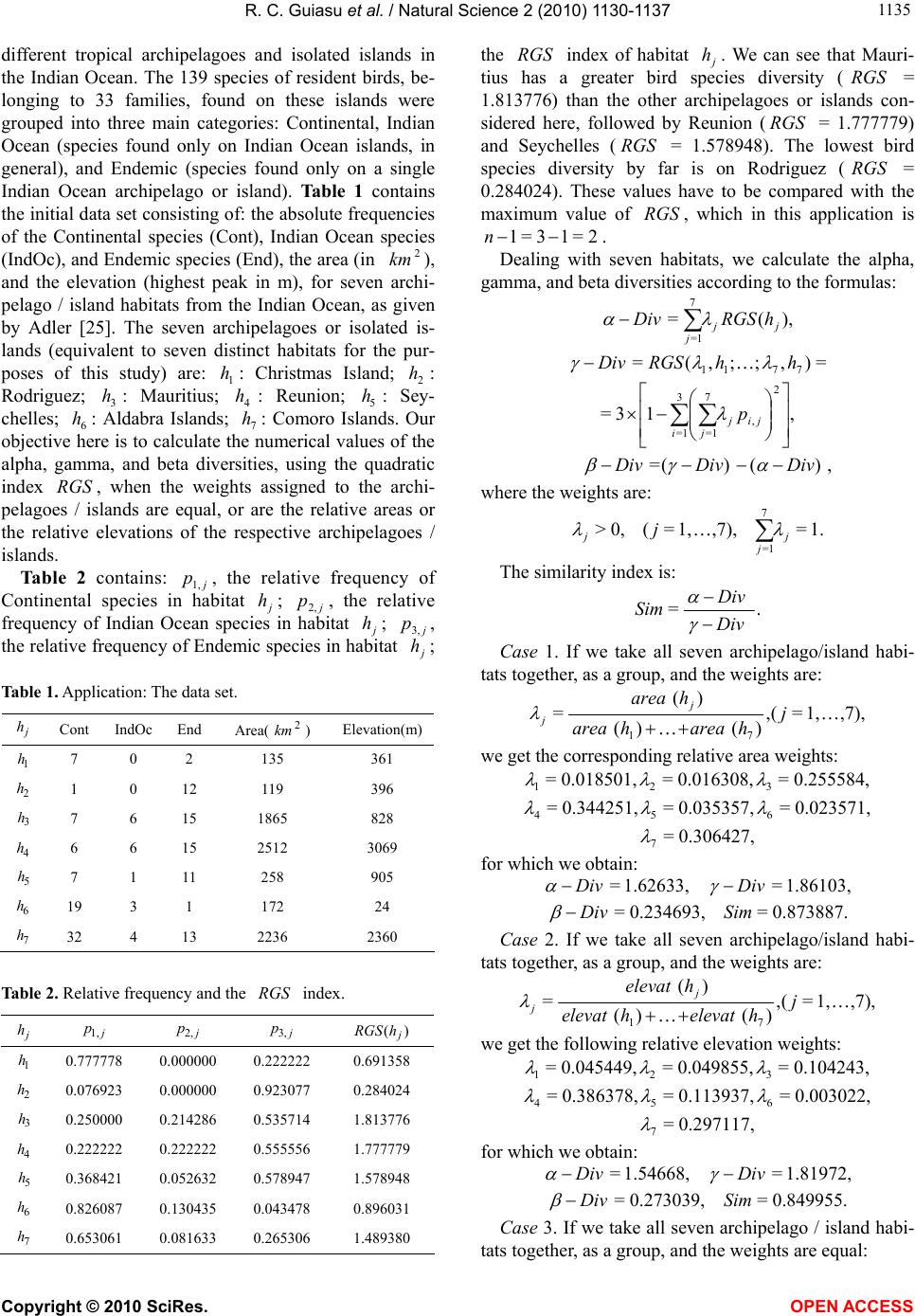

R. C. Guiasu et al. / Natural Science 2 (2010) 1130-1137
113
1135
different tropical archipelagoes and isolated islands in
the Indian Ocean. The 139 species of resident birds, be-
longing to 33 families, found on these islands were
grouped into three main categories: Continental, Indian
Ocean (species found only on Indian Ocean islands, in
general), and Endemic (species found only on a single
Indian Ocean archipelago or island). Table 1 contains
the initial data set consisting of: the absolute frequencies
of the Continental species (Cont), Indian Ocean species
(IndOc), and Endemic species (End), the area (in 2
km ),
and the elevation (highest peak in m), for seven archi-
pelago / island habitats from the Indian Ocean, as given
by Adler [25]. The seven archipelagoes or isolated is-
lands (equivalent to seven distinct habitats for the pur-
poses of this study) are: 1
h: Christmas Island; 2 h:
Rodriguez; 3
h: Mauritius; 4 h: Reunion; 5 h: Sey-
chelles; 6 h: Aldabra Islands; 7 h: Comoro Islands. Our
objective here is to calculate the numerical values of the
alpha, gamma, and beta diversities, using the quadratic
index RGS , when the weights assigned to the archi-
pelagoes / islands are equal, or are the relative areas or
the relative elevations of the respective archipelagoes /
islands.
Table 2 contains: j p1,, the relative frequency of
Continental species in habitat j h; j p2, , the relative
frequency of Indian Ocean species in habitat j h; j p3, ,
the relative frequency of Endemic species in habitat j h;
Table 1. Application: The data set.
j
h Cont IndOc End Area( 2
km ) Elevation(m)
1
h 7 0 2 135 361
2
h 1 0 12 119 396
3
h 7 6 15 1865 828
4
h 6 6 15 2512 3069
5
h 7 1 11 258 905
6
h 19 3 1 172 24
7
h 32 4 13 2236 2360
Table 2. Relative frequency and the RGS index.
j
h j
p1, j p2, j p3, )(j
hRGS
1
h 0.777778 0.000000 0.222222 0.691358
2
h 0.076923 0.000000 0.923077 0.284024
3
h 0.250000 0.214286 0.535714 1.813776
4
h 0.222222 0.222222 0.555556 1.777779
5
h 0.368421 0.052632 0.578947 1.578948
6
h 0.826087 0.130435 0.043478 0.896031
7
h 0.653061 0.081633 0.265306 1.489380
the RGS index of habitat j h. We can see that Mauri-
tius has a greater bird species diversity (RGS =
1.813776) than the other archipelagoes or islands con-
sidered here, followed by Reunion (RGS = 1.777779)
and Seychelles (RGS = 1.578948). The lowest bird
species diversity by far is on Rodriguez (RGS =
0.284024). These values have to be compared with the
maximum value of RGS , which in this application is
2=13=1


n.
Dealing with seven habitats, we calculate the alpha,
gamma, and beta diversities according to the formulas:
),(=
7
1=
jj
j
hRGSDiv 


=),;;,(=7711 hhRGSDiv





,13=
2
,
7
1=
3
1= 















  jij
ji
p 
,)()(=DivDivDiv 





where the weights are:
1.=,7),1,=(0,>
7
1=
j
j
jj



The similarity index is:
.= Div
Div
Sim 



Case 1. If we take all seven archipelago/island habi-
tats together, as a group, and the weights are:
,7),1,=(,
)()(
)(
=
71

j hareaharea
harea j
j

we get the corresponding relative area weights:
0.255584,=0.016308,=0.018501,=321



0.023571,=0.035357,=0.344251,=654



0.306427,=
7

for which we obtain:
1.86103,=1.62633,= DivDiv 



0.873887.=0.234693,=SimDiv


Case 2. If we take all seven archipelago/island habi-
tats together, as a group, and the weights are:
,7),1,=(,
)()(
)(
=
71

j helevathelevat
helevat j
j

we get the following relative elevation weights:
0.104243,=0.049855,=0.045449,=321



0.003022,=0.113937,=0.386378,=654



0.297117,=
7

for which we obtain:
1.81972,=1.54668,=DivDiv 



0.849955.=0.273039,=SimDiv


Case 3. If we take all seven archipelago / island habi-
tats together, as a group, and the weights are equal:

R. C. Guiasu et al. / Natural Science 2 (2010) 1130-1137
1136
,7),1,=(,
7
1
=j
j

we obtain the average values:
1.75528,=1.21876,= DivDiv  
0.694339.=0.536528,= SimDiv 
Generally, for islands or habitat islands found in a
similar geographic region, species diversity tends to be
greater on the island or habitat island with a larger area
or a higher elevation. The above numerical results ob-
tained by using RGS as the main mathematical tool,
show that by taking the area and elevation into account,
in this order, the alpha and gamma species diversities
increase whereas the beta species diversity decreases
compared to what happens when we calculate the mean
within-habitat and between-habitat species diversity ig-
noring such factors. Calculating the alpha, beta, and
gamma species diversities by using the relative areas and
the relative elevation as weights, we compensate for the
lack of homogeneity of the habitats with respect to such
essential factors which influence species diversity.
5. CONCLUSIONS
The Gini-Simpson index for species diversity is very
popular with many ecologists. Recently, however, Jost
[18,19,24] showed that this index does not behave well
when the number of species is large and is not suitable
for use in the computation of the between-habitat species
diversity, also called the beta diversity. As a result, Jost
pleaded in favour of abandoning the Gini-Simpson index
and replacing the additive partitioning of species diver-
sity, prefered by many ecologists, with the multiplicative
partitioning. The objective of this paper is to show that
the additive partitioning of species diversity may be
preserved but the classic Gini-Simpson index of diver-
sity should be replaced by the Rich-Gini-Simpson index,
abbreviated as RGS , which behaves well when the
number of species is large, while keeping the useful
basic properties of the classic Gini-Simpson index un-
changed. The properties of the RGS index and its use
in the additive partitioning of the species diversity are
analyzed. RGS is also applied to data on the avifaunal
diversity on several tropical Indian Ocean islands (using
some of the numerical data obtained by Adler [25]). The
application shows that by using the RGS index as a
mathematical tool and introducing weights directly pro-
portional with the areas or elevation of the habitats (in
this order), the within-habitat species diversity and the
total species diversity increase while the between-
habitat species diversity decreases compared to what
happens when we calculate the mean within-habitat and
between-habitat species diversities ignoring such im-
portant factors.
REFERENCES
[1] Sarkar, S. (2007) From ecological diversity to biodiver-
sity. In: Hull, D.L. and Ruse, M. Eds., The Philosophy of
Biology, Cambridge University Press, Cambridge, 388-
409.
[2] Gini, C. (1912) Variabilità e mutabilità. In: Pizetti, E. and
Salvemini, T. Eds., Rome: Libreria Eredi Virgilio Veschi,
Memorie di metodologica statistica.
[3] Simpson, E.H. (1949) Measurement of diversity. Nature,
163, 688.
[4] Shannon, C.E. (1948) A mathematical theory of commu-
nication. Bell System Technical Journal, 27, 379-423, 623-
656.
[5] Boltzmann, L. (1896) Vorlesungen über Gastheorie. J.A.
Barth edition, Akademische Druck-u, Leipzig.
[6] Pielou, E.C. (1966) Shannon’s formula as a measure of
specific diversity: Its use and misuse. American Natural-
ist, 100, 463-465.
[7] Pielou, E.C. (1966) Species-diversity and pattern-diversity
in the study of ecological succession. Journal of Theo-
retical Biology, 10, 370-383.
[8] Pielou, E.C. (1975) Ecological Diversity. Wiley, New York.
[9] Guiasu, S. (1977) Information Theory with Applications.
McGraw-Hill, New York.
[10] Patil, G.P. and Taillie, C. (1982) Diversity as a concept
and its measurement. Journal of American Statistical
Association, 77, 548-567.
[11] Harper, J.L. and Hawksworth, D.L. (1994) Biodiversity:
Measurement and estimation. Philosophical Transactions:
Biological Sciences, 345, 5-12.
[12] Magnussen, S. and Boyle, T.J.B. (1995) Estimating sam-
ple size for inference about the Shannon-Weaver and the
Simpson indices of species diversity. Forest Ecology and
Management, 78, 71-84.
[13] Krebs, C.J. (2001) Ecology: The experimental analysis of
distribution and abundance. 5th Edition, Benjamin Cum-
mings, San Francisco.
[14] Guiasu, R.C. and Guiasu, S. (2003) Conditional and weight-
ed measures of ecological diversity. International Jour-
nal of Uncertainty, Fuzziness and Knowledge-Based Sys-
tems, 11, 283-300.
[15] Guiasu, R.C. and Guiasu, S. (2003) Entropy in ecology
and ethology. Nova Science Publishers, New York.
[16] Magurran, A.E. (2004) Measuring biological diversity.
Blackwell Publishing, Malden MA.
[17] Maclaurin, J. and Sterelny, K. (2008) What is biodiver-
sity? University of Chicago Press, Chicago and London.
[18] Jost, L. (2006) Entropy and diversity. Oikos, 113, 363-
375.
[19] Jost, L. (2007) Partitioning diversity into independent
alpha and beta components. Ecology, 88, 2427-2439.
[20] Hill, M. (1973) Diversity and evenness. A unifying nota-
tion and its consequences. Ecology, 54, 427-432.
[21] Rényi, A. (1961) On measures of entropy and informa-
tion. In: Neyman, J. Ed., Fourth Berkeley Symposium on
Mathematical Statistics and Probability, Berkeley, 547-
561.

R. C. Guiasu et al. / Natural Science 2 (2010) 1130-1137
113
1137
[22] Hoffmann, S. and Hoffmann, A. (2008) Is there a “true”
diversity? Ecological Economics, 65, 213-215.
[23] Ricotta, C. (2005) Through the jungle of biological di-
versity. Acta Biotheoretica, 53, 29-38.
[24] Jost, L. (2009) Mismeasuring biological diversity: Re-
sponse to Hoffmann and Hoffmann. Ecological Econom-
ics, 68, 925-928.
[25] Adler, G.H. (1994) Avifaunal diversity and endemism on
tropical Indian Ocean islands. Journal of Biogeography,
21, 85-95.
[26] MacArthur, R.H. (1965) Patterns of species diversity. Bio-
logical Review, 40, 510-533.
[27] MacArthur, R.H., Recher, H. and Cody, M. (1966) On
the relation between habitat selection and species diver-
sity. American Naturalist, 100, 319-332.
[28] MacArthur, R.H. and Wilson, E.O. (1967) The theory of
island biogeography. Princeton University Press, Princeton.
[29] Rao, C.R. (1982) Diversity and dissimilarity coefficients:
A unified approach. Theoretical Population Biology, 21,
24-43.
[30] Whittaker, R.H. (1972) Evolution and measurement of
species diversity. Taxon, 21, 213-251.
[31] Whittaker, R.H. (1977) Evolution of species diversity in
land communities. In: Hecht, M.K. and Steere, B.W.N.C.
Eds., Evolutionary Biology, Plenum Press, New York, 10,
1-67.
[32] Harrison, S. and Quinn, J. (2006) The importance of

-
diversity. In: Groom, M.J., Meffe, G.K. and Carroll, C.R.
Eds., Principles of Conservation Biology, 3rd Edition,
Sinauer Associates Inc. Publishers, Sunderland, 44-45.
[33] Routledge, R.D. (1977) On Whittaker’s components of
diversity. Ecology, 58, 1120-1127.
[34] Routledge, R.D. (1979) Niche metrics and diversity com-
ponents. Oecologia, 43, 121-124.
[35] Allan, J.D. (1975) Components of diversity. Oecologia,
18, 359-367.
[36] Lande, R. (1996) Statistics and partitioning of species di-
versity and similarity among multiple communities. Oikos,
76, 5-13.
[37] Wagner, H.H., Wildi, O. and Ewald, K.C. (2000) Addi-
tive partitioning of plant species diversity in an agricul-
tural mosaic landscape. Landscape Ecology, 15, 219-227.
[38] Veech, J.A., Summerville, K.S., Crist, T.O. and Gering,
J.C. (2002) The additive partioning of species diversity:
Recent revival of an old idea. Oikos, 99, 3-9.
[39] Tramer, E.J. (1969) Bird species diversity: Components
of Shannon’s formula. Ecology, 50, 927-929.
[40] Fager, E.W. (1972) Diversity: A sampling study. Ameri-
can Naturalist, 106, 293-310.
[41] Brown, J.H. and Lomolino, M.V. (1998) Biogeography.
2nd Edition, Sinauer Associates Inc. Publishers, Sunder-
land.
[42] Stirling, G. and Wilsey, B. (2001) Empirical relationships
between species richness, evenness, and proportional di-
versity. American Naturalist, 158, 286-299.
[43] Cox, C.B. and Moore, P.D. (2005) Biogeography: An
ecological and evolutionary approach. 7th Edition, Black-
well Publishing, Oxford.
[44] Quammen, D. (1997) The song of the Dodo-Island bio-
geography in an Age of Extinction. Simon & Schuster
Inc., New York.
[45] Powledge, F. (2003) Island biogeography’s lasting impact.
BioScience, 53, 1032-1038.