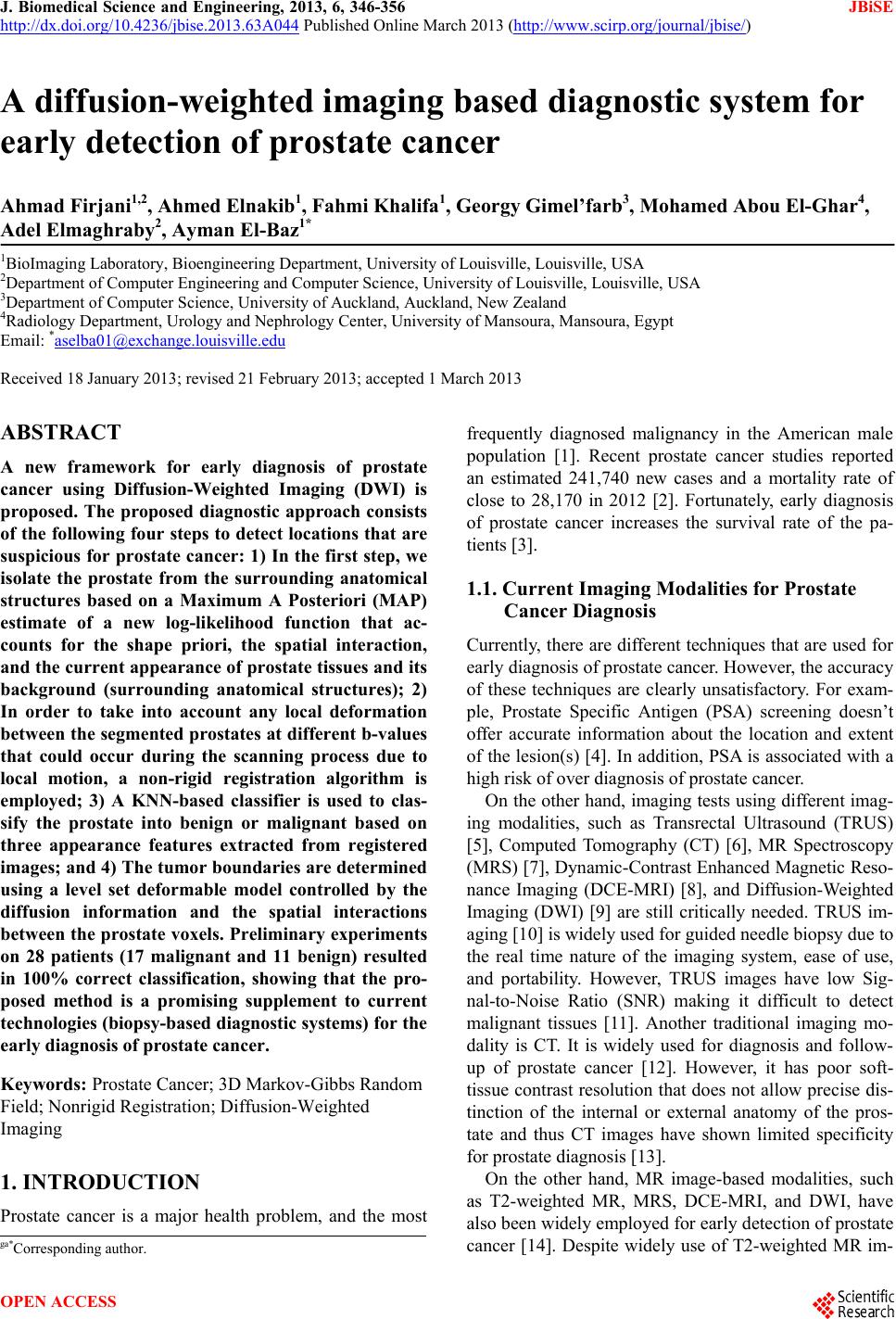
J. Biomedical Science and Engineering, 2013, 6, 346-356 JBiSE
http://dx.doi.org/10.4236/jbise.2013.63A044 Published Online March 2013 (http://www.scirp.org/journal/jbise/)
A diffusion-weighted imaging based diagnostic system for
early detection of prostate cancer
Ahmad Firjani1,2, Ahmed Elnakib1, Fahmi Khalifa1, Georgy Gimel’farb3, Mohamed Abou El-Ghar4,
Adel Elmaghraby2, Ayman El-Baz1*
1BioImaging Laboratory, Bioengineering Department, University of Louisville, Louisville, USA
2Department of Computer Engineering and Computer Science, University of Louisville, Louisville, USA
3Department of Computer Science, University of Auckland, Auckland, New Zealand
4Radiology Department, Urology and Nephrology Center, University of Mansoura, Mansoura, Egypt
Received 18 January 2013; revised 21 February 2013; accepted 1 March 2013
ABSTRACT
A new framework for early diagnosis of prostate
cancer using Diffusion-Weighted Imaging (DWI) is
proposed. The proposed diagnostic approach consists
of the following four steps to detect locations that are
suspicious for prostate cancer: 1) In the first step, we
isolate the prostate from the surrounding anatomical
structures based on a Maximum A Posteriori (MAP)
estimate of a new log-likelihood function that ac-
counts for the shape priori, the spatial interaction,
and the current appearance of prostate tissues and its
background (surrounding anatomical structures); 2)
In order to take into account any local deformation
between the segmented prostates at different b-values
that could occur during the scanning process due to
local motion, a non-rigid registration algorithm is
employed; 3) A KNN-based classifier is used to clas-
sify the prostate into benign or malignant based on
three appearance features extracted from registered
images; and 4) The tumor boundaries are determined
using a level set deformable model controlled by the
diffusion information and the spatial interactions
between the prostate voxels. Preliminary experiments
on 28 patients (17 malignant and 11 benign) resulted
in 100% correct classification, showing that the pro-
posed method is a promising supplement to current
technologies (biopsy-based diagnostic systems) for the
early diagnosis of prostate cancer.
Keywords: Prostate Cancer; 3D Markov-Gibbs Random
Field; Nonrigid Registration; Diffusion-Weighted
Imaging
1. INTRODUCTION
Prostate cancer is a major health problem, and the most
frequently diagnosed malignancy in the American male
population [1]. Recent prostate cancer studies reported
an estimated 241,740 new cases and a mortality rate of
close to 28,170 in 2012 [2]. Fortunately, early diagnosis
of prostate cancer increases the survival rate of the pa-
tients [3].
1.1. Current Imaging Modalities for Prostate
Cancer Diagnosis
Currently, there are different techniques that are used for
early diagnosis of prostate cancer. However, the accuracy
of these techniques are clearly unsatisfactory. For exam-
ple, Prostate Specific Antigen (PSA) screening doesn’t
offer accurate information about the location and extent
of the lesion(s) [4]. In add ition, PSA is associated with a
high risk of over di agnosis of p rostate can c er.
On the other hand, imaging tests using different imag-
ing modalities, such as Transrectal Ultrasound (TRUS)
[5], Computed Tomography (CT) [6], MR Spectroscopy
(MRS) [7], Dynamic-Contrast Enhanced Magnetic Reso-
nance Imaging (DCE-MRI) [8], and Diffusion-Weighted
Imaging (DWI) [9] are still critically needed. TRUS im-
aging [10] is widely used for guided needle biopsy due to
the real time nature of the imaging system, ease of use,
and portability. However, TRUS images have low Sig-
nal-to-Noise Ratio (SNR) making it difficult to detect
malignant tissues [11]. Another traditional imaging mo-
dality is CT. It is widely used for diagnosis and follow-
up of prostate cancer [12]. However, it has poor soft-
tissue contrast resolution that does not allow precise dis-
tinction of the internal or external anatomy of the pros-
tate and thus CT images have shown limited specificity
for prostate dia gn osi s [1 3] .
On the other hand, MR image-based modalities, such
as T2-weighted MR, MRS, DCE-MRI, and DWI, have
also been widely employed for early detection of prostate
cancer [14]. Despite widely use of T2-weighted MR im-
ga*Corresponding author.

A. Firjani et al. / J. Biomedical Science and Engineering 6 (2013) 346-356 347
aging for prostate cancer, the technique is limited by un-
satisfactory sensitivity and specificity for cancer detec-
tion and localization [15]. To improve the diagnostic
performance of MR imaging in evaluations for prostate
cancer, various other techniques have been applied. MRS
provides metabolic information about prostate tissue by
demonstrating the relative concentration of chemical
compounds. However, MRS has its own limitations, such
as the need of an additional software and longer acquisi-
tion time [16], which lead to increased costs and de-
creased throughput. Furthermore, MRS suffers from lack
of spatial resolution. In add ition, signal from periprostatic
fat and seminal vesicles can distort spectral waveforms
[14]. DCE-MRI has been recently suggested for im-
proved visualization and localization of the prostate can-
cer [17]. It provides valuable pathologic and anatomical
information. However, DCE-MRI has the drawback of
intravenous contrast agent (e.g., gadolinium) administra-
tion which is harmful to the kidney [18] and requires a
longer setup time.
Recently, DWI has emerged as an imaging modality
that has shown more capabilities in determining the size
and the shape of the prostate gland and localizing the
cancer foci [19]. DWI is non-contrast functional imaging
technique, whereby the image contrast is determined by
the random microscopic motion of water protons, i.e., the
Brownian motion [19]. Moreover, DWI has the distinct
advantage of being acquired very rapidly, without the use
of any intravenous contrast material or specialized hard-
ware, and this is the main motivation behind this work.
1.2. Clinical Studies for Prostate Cancer
Diagnosis Using DWI
In recent years, a growing number of clinical studies [19-
30] have evaluated the utility of DWI, either in combina-
tion with or in comparison with other MRI techniques,
for the detection of prostate cancer. These studies have
reported various sensitivities and specificities of cancer
diagnosis.
Earlier studies [19,20] have investigated the abilities
of DWI for prostate cancer diagnosis using an endorectal
coil. However, the reported results demonstrated low
diagnostic sensitivity. To increase the sensitivity of di-
agnosis, Shimofusa et al. [21] suggested the addition of
strong magnetic field gradient pulses (b-values) to the
pulse sequence instead of using endorectal coil. In their
study [21], they detected the tumor in the central zone of
the prostate in five of eight total patients using DWI with
strong magnetic field gradient pulses. Alternatively, the
compared diagnostic results with T2-weighted imaging,
detected the tumor only in one of the eight patients.
Since then, DWI was used for the detection of cancerous
tissue in later studies [22-30]. For example, Tan et al. [30]
compared the performance of T2-weighted MRI, DCE-
MRI, and DWI for the detection of cancer within the
prostate gland. In their study they reported that DWI
alone showed better specificity than DCE-MRI alone. It
is also showed better overall specificity than combined
DWI and T2-weighted imaging.
To the best of our knowledge, there are a very limited
number of image-based approaches for automated com-
puter-aided diagnosis of prostate cancer using DWI.
These related works are discussed in the following sec-
tion.
1.3. Image-Based Computer-Aided Diagnostic
(CAD) Systems for Prostate Cancer
Detection
In literature, a limited number of CAD systems for pros-
tate cancer diagnosis have been proposed. For example,
Chan et al. [31] proposed an in-vivo CAD system using
multimodal MRI to estimate malignancy likelihood in
the peripheral zone. They constructed statistical maps
from T2-weighted MRI, DWI, and Proton Density (PD)
images. These statistic maps were combined with tex-
tural and anatomical features of prostate cancer areas in
order to detect the cancerous regions. However, this
study doesn’t include benign regions. Huisman et al. [32]
developed a CAD system for prostate lesion classifica-
tion using a Hessian-based blob detection algorithm [33].
Results showed an accuracy of 92% in classification
within the peripheral region and an accuracy of 83% in
classification within transitional zones of the prostate.
However, their study focused on the peripheral and tran-
sitional zones of the prostate gland and excluded central
zones in which up to 30% of prostate cancers can occur.
Viswanath et al. [34] generated similar likelihood
maps by combining information from multimodal MR
images using mathematical descriptors. Their study
showed, on a voxel basis, that the discrimination be-
tween benign and malignant tissue is feasible with good
performances. The unsupervised classification by k-
means clustering achieved an accuracy of 77%. Unfor-
tunately, th e corresponding slice still needs to be selected
between different modality. A study by Langer et al. [35]
focused on the peripheral zone of the prostate gland and
excluded the central and transitional zones. However,
detailed anatomic studies have suggested that 70% of
cancers arise in the peripheral zone of the prostate, but
up to 30% of prostate cancers occur between transition
zones and the central zone of the prostate [36].
To increase the sensitivity of diagnosis, accurate de-
lineation of the prostate region is mandatory. Basically,
manual outlining of the prostate borders is the most ac-
curate segmentation that en ables pr ecise determination o f
the prostate volume. However, it is prohibitively time

A. Firjani et al. / J. Biomedical Science and Engineering 6 (2013) 346-356 348
consuming and is prone to intra- and inter-observer vari-
ability. Traditional edge detection methods (e.g., [39])
are unable to extract the correct boundaries of the pros-
tate since the gray-level distributions of the prostate and
the surrounding organs are hardly distinguishable. There-
fore, other automated segmentation methods are desir-
able. However, multiple challenges stemming from 1)
the large variations of prostate shape within a specific
time series as well as across subjects; 2) lack of strong
edges and diffused prostate boundaries; and 3) the simi-
lar signal-intensity profile of the prostate and surround-
ing tissues, complicates the segmentation process.
The most successful known approaches (e.g., [37-45])
have addressed the segmentation challenges of the pros-
tate by modeling object appearance and shape. In par-
ticular, Zhu et al. [40] used a combination of an Active
Shape Model (ASM) and 3D statistical shape modeling
to segment the prostate. Toth et al. [41] presented an al-
gorithm for the automatic segmentation of the pros tate in
multi-modal MRI. Their algorithm starts by isolating the
Region-Of-Interest (ROI) from MRS data. Then, an ASM
within the ROI is used to obtain the final segmentation.
Klein et al. [42] presented an atlas-based segmentation
approach to extract the prostate from MR images. The
segmentation of the prostate is obtained as the average of
the best-matched registered atlas set to the test image
(image to be segmented). Recently, Vikal et al. [43] used
a priori knowledge of prostate shape to detect the contour
in each slice and then refined them to form a 3D prostate
surface. Martin et al. [44] developed an atlas-based ap-
proach for segmenting the prostate from 3D MR images
by mapping probabilistic anatomical atlas to the test im-
age. The resulting map is used to constrain a deformable
model-based segmentation framework.
1.4. Current Limitations and Motivation for Our
Proposal
The above-mentioned CAD systems for analyzing DWI
are not sufficiently accurate and reliable for several rea-
sons:
1) The majority of CAD systems used multimodal
MRI which is cost inefficient [45].
2) The majority of these studies require user interac-
tion to select a ROI (a small window) around the pro state.
Unfortunately, such approaches not only prone to inter-
observer variability, but also ROI selection biases the
final decision by over- or under-estimating the problem
in the entire graft, just as with biopsy.
3) Automated prostate segmentation methods have one
of the following limitations:
 Deformable model-based methods without adequate
appearance and shape priors fail under excessive
noise, poor resolution, diffused boundaries, or oc-
cluded shapes in the images;
 Segmentation based only on the shape prior still re-
sults in large errors caused by discontinuities in ob-
ject boundaries, large image noise, and other inho-
mogeneities;
 Parametric shape-based models are unsuitable for
discontinuous prostate objects due to a very small
number of distinct landmarks.
4) The majority of CADs assumes that the prostates
(prostate contours) remain exactly the same from scan to
scan. However, prostate contours may not always exactly
match due to patient movement or breathing effects;
therefore, image registration schemes should be applied
first before ROI selection/segmentation.
To overcome these limitations, we propose an auto-
matic framework for analyzing DWI images building on
our previous work in [46-48]. The proposed approach
consists of the following steps as shown in Figur e 1:
1) Segmentation of the prostate from DWI (Section
2.1) based on a Maximum a Posteriori (MAP) estimate
of a new likelihood function that accounts for both ap-
pearance features of the prostate (Section 2.1.1) and th eir
3D spatial voxel interactions (Section 2.1.2), as well as a
3D shape prior (Section 2.1.3).
2) A non-rigid registration approach is employed to
account for any local deformation that could occur in the
prostate during the scanning process based on the solu-
tion of the Laplace equation (Section 2.3).
3) KNN classifier to classify the prostate into benign
or malignant based on three appearance features ex-
tracted from registered images (Section 3.2).
2. MATERIALS AND METHODS
In this paper we introduce a new, automated, and non-
invasive framework for early diagnosis of prostate cancer
from DWI. Figure 1 demonstrates the steps of the pro-
posed CAD system. Below, we will illustrate each of
these steps.
2.1. Segmentation of the Prostate Using a Joint
MGRF Model
The segmentation of the prostate is a challenge, since the
gray-level distribution of the prostate and surrounding
organs is not highly distinguishable and because of the
anatomical complexity of prostate. This stage proposes a
powerful framework for prostate segmentation based on
a learned shape model and an identifiable joint Markov-
Gibbs Random Field (MGRF) model of DWI and “ob-
ject-background” region maps.
The joint-MGRF model is fundamentally a model that
relates the joint probability of an image and its object-
background region map, to geometric structure and to the
nergy of repeated patterns within the image. The basic e

A. Firjani et al. / J. Biomedical Science and Engineering 6 (2013) 346-356 349
Figure 1. Flowchart of the proposed CAD system for automatic detection of cancer from 3D DWI.
theory behind such models is that they assume that the
signals associated with each pixel depend on the signals
of the neighboring pixels, and thus explicitly take into
account their spatial interactions, and other features, such
as the shape.
Let , , and

0,1, ,1QQ

,ob bgL



0, 1U
be a set of integer gray-level, a set of object (“ob”)
and background (“bg”) labels, and a unit interval, respec-
tively. Let a 3D arithmetic grid
Q
 

,,:0,1, ,1;
0,1, ,1;0,1, ,1
xyz xX
yYzZ




R

Figure 2. Aligning a 3-D joint Markov-Gibbs random field
model with shape prior of DWI.
support a grayscale DWI and their binary
region maps , and probabilistic shape model
. The shape model allows for registering
(aligning) 3D prostate DWI. The DWI data
:gR Q
:mR L
:sR U
g
and their
region maps are described with a joint probability
model [49,50]:
m
shape model provides the voxel-wise object and back-
ground probabilities be ing used, together with the condi-
tional image intensity model

P

g
m, to build an initial
region map. The final Bayesian segmentation is per-
formed using the identified joint MGRF model of the
DWI and region maps.



,h PPP
g
m
g
mm (1)
where is a 2nd-order MGRF of region maps and

h
Pm

P
g
m is a conditionally independent random field of
image intensities given the map. The map model 2.1.1. Con dition al Intensity M o d el
The specific visual appearance of the prostate in each
data set to be segmented is taken in to account by model-
ing a marginal gray level distribution with a Linear Com-
bination of Discrete Gaussians (LCDG) [50,51]. Close
approximation with LCDG separates each factor of the
joint empirical gray level distribution,
 
hs
PPPmm

s
Pm
m has two parts: a shape prior prob-
ability being a spatially varian t independen t random field
of region labels , for a set of co-aligned training
DWI data, and a 2nd-order MGRF model



Pm of a
spatially homogeneous evolving map.




,x y
Pp g

,mix xy R, into two (object and back-
ground) components,
The Bayesian MAP estimate of the map, given the
DWI data


,argmax,gmL gmm
 maximize the log-
likelihoo d f unction:
g




;,andq   QLpq . The
LCDG modeling restores transitions between these
components more accurately than conventional mixtures
of only positive Gaussians, thus yielding a better initial
region map formed by voxel-wise classification of the
image gray values, the similar intensity profile of the
prostate and surrounding tissues.
 

 
,log log
h
LP P
g
m
g
mm
In this work we focus on accu rate identification of the
spatial interaction between the prostate voxels


Pm,
and the intensity distribution for the prostate tissues,

P

g
m, and the prior distribution of the pros-
tate shape, as shown in Figure 2.

s
Pm2.1.2. Spatial Voxel In te raction M odel
In order to overcome noise effect and to ensure the ho-
mogeneity of the segmentation, spatially voxel interac-
To perform the initial prostate segmentation, a given
3D DWI is aligned to one of the training 3D DWI. The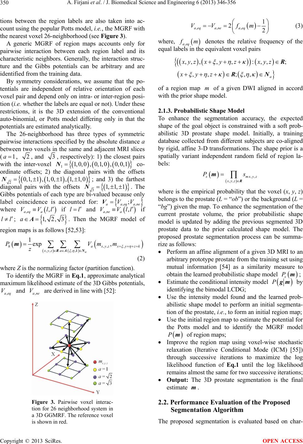

A. Firjani et al. / J. Biomedical Science and Engineering 6 (2013) 346-356 350
tions between the region labels are also taken into ac-
count using the popular Potts model, i.e., the MGRF with
the nearest voxel 2 6-neighborhood (see Figure 3).
A generic MGRF of region maps accounts only for
pairwise interaction between each region label and its
characteristic neighbors. Generally, the interaction struc-
ture and the Gibbs potentials can be arbitrary and are
identified from the training data.
By symmetry considerations, we assume that the po-
tentials are independent of relative orientation of each
voxel pair and depend only on intra- or inter-region posi-
tion (i.e. whether the labels are equal or not). Under these
restrictions, it is the 3D extension of the conventional
auto-binomial, or Potts model differing only in that the
potentials are estimated analyt ically.
The 26-neighborhood has three types of symmetric
pairwise interaction s specified by the absolute distan ce a
between two voxels in the same and adjacent MRI slices
(, 1a2, and 3, respectively): 1) the closest pairs
with the inter-voxel co-
ordinate offsets; 2) the diagonal pairs with the offsets


11,0,0, 0,1,0 , 0,0,1N

0,1,1,1, 0N
 
, 1,1, 1,0
2; and 3) the farthest
diagonal pairs with the offsets
 
3. The
Gibbs potentials of each type are bi-valued because only
label coincidence is accounted for:
where if l
1, 1, 1

;
aaeq
VVV
N

,, aeqa
VVll

l

,,ane

 and


ll
,, ane a
VV

 if
ll;

1,2, 3aA. Then the MGRF model of
region maps is as follows [52,53]:
 

,, ,
,, ,,
1exp ,
a
haxy
xyzak
PVm
z



 
 
RA N
m

zxyzk
m
(2)
where Z is the normalizing factor (partition function).
To id en tif y th e MGR F in Eq.1, approximate analytical
maximum likelihood estimate of th e 3D Gibbs potentials,
and are derived in line with [52]:
,aeq
V,ane V
Figure 3. Pairwise voxel interac-
tion for 26 neighborhood system in
a 3D GGMRF. The reference voxel
is shown in red.

,,, 1
22
aeqaneaeq
VV fm

 




(3)
where,


,aeq
f
m denotes the relative frequency of the
equal labels in the equivalent voxel pairs
 

 



,, ,,,: ,,;
,,;,, a
xyz xyzxyz
xyz

 
 
 
R
RN
of a region map of a given DWI aligned in accord
with the prior shape model.
m
2.1.3. Probabilistic Shape Model
To enhance the segmentation accuracy, the expected
shape of the goal object is constrained with a soft prob-
abilistic 3D prostate shape model. Initially, a training
database collected from different subjects are co-aligned
by rigid, affine 3-D transformations. The shape prior is a
spatially variant independent random field of region la-
bels:



,,
,,
s
mx y z
xyz
Ps

R m
where is the empirical probability that the voxel (x, y, z)
belongs to the prostate (L = “ob”) or the backgro und ( L =
“bg”) given the map. To enhance the segmentation of the
current prostate volume, the prior probabilistic shape
model is updated by adding the previous segmented 3D
prostate data to the prior calculated shape model. The
proposed prostate segmentation process can be summa-
rize as follows:
 Perform an affine alignment of a given 3D MRI to an
arbitrary prot ot ype prost ate f rom t he traini ng set usi ng
mutual information [54] as a similarity measure to
obtain the learned probabilistic shape model


s
Pm;
 Estimate the conditional intensity model


Pgm by
identifying the bimodal LCDG;
 Use the intensity model found and the learned prob-
abilistic shape model to perform an initial segmenta-
tion of the pros t a t e , i.e., to form an initial region map;
 Use the initial region map to estimate the potential for
the Potts model and to identify the MGRF model


Pm of region maps;
 Improve the region map using voxel-wise stochastic
relaxation (Iterative Conditional Mode (ICM) [55])
through successive iterations to maximize the log
likelihood function of Eq.1 until the log likelihood
remains almost the same for two successive iterations;
 Output: The 3D prostate segmentation is the final
estimate m.
2.2. Performance Evaluation of the Proposed
Segmentation Algorithm
The proposed segmentation is evaluated based on char-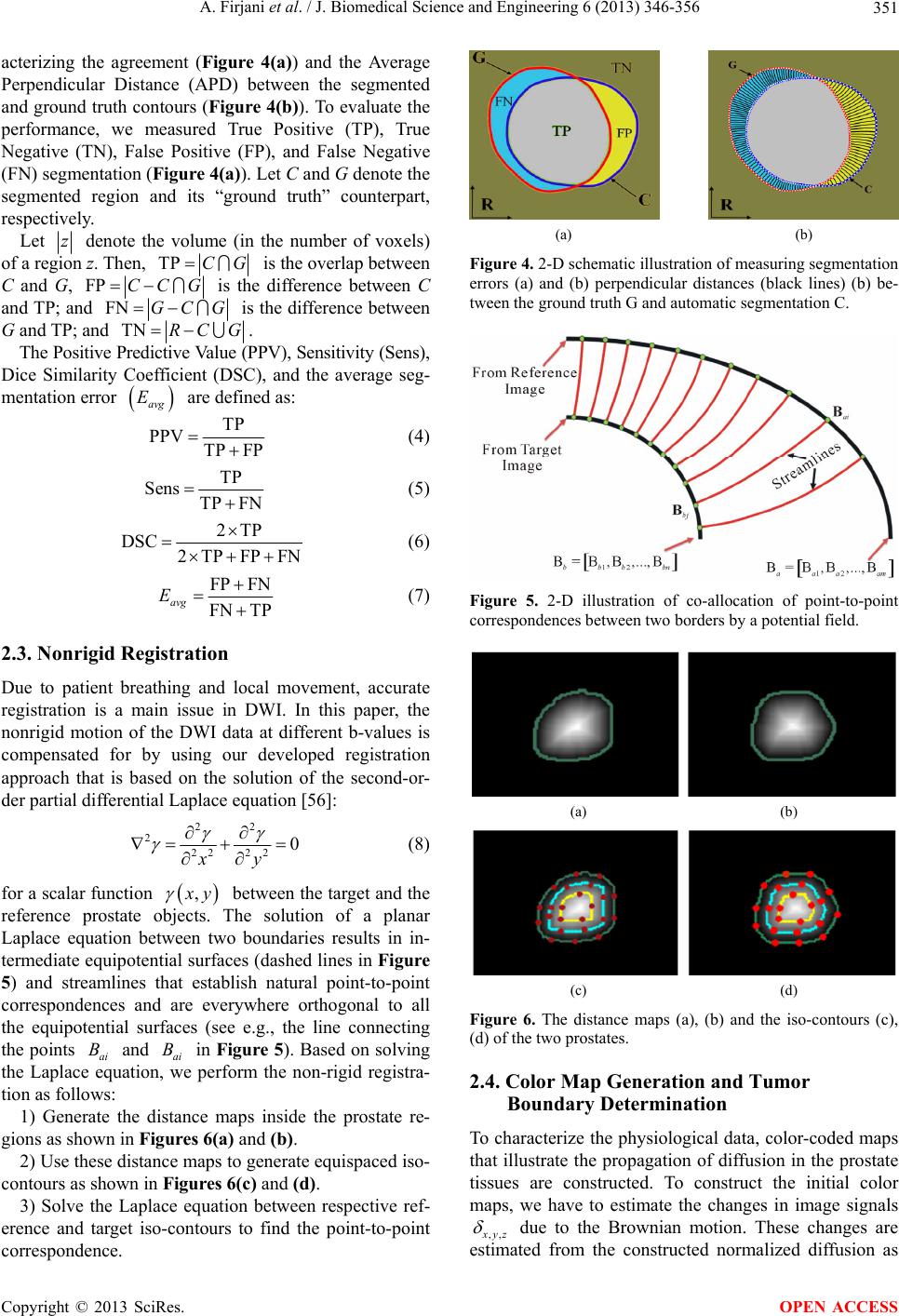

A. Firjani et al. / J. Biomedical Science and Engineering 6 (2013) 346-356 351
acterizing the agreement (Figure 4(a)) and the Average
Perpendicular Distance (APD) between the segmented
and ground truth contours (Figure 4(b)). To evaluate the
performance, we measured True Positive (TP), True
Negative (TN), False Positive (FP), and False Negative
(FN) segmentation (Figure 4(a)). Let C and G denote the
segmented region and its “ground truth” counterpart,
respectively.
Let z denote the volume (in the number of voxels)
of a region z. Then, TPCG is the overlap between
C and G, FP CCG is the difference between C
and TP; and FNGC G is the differe nce between
G and TP; and TNRC G.
The Positive Predictiv e Value (PPV), Sensitivity (Sens),
Dice Similarity Coefficient (DSC), and the average seg-
mentation error are defined as:

avg
E

TP
PPV TP FP  (4)
TP
Sens TP FN  (5)
2TP
DSC 2TPFPFN

 (6)
FP FN
FN TP
avg
E

 (7)
2.3. Nonrigid Registration
Due to patient breathing and local movement, accurate
registration is a main issue in DWI. In this paper, the
nonrigid motion of the DWI data at different b-values is
compensated for by using our developed registration
approach that is based on the solution of the second-or-
der partial differential Laplace equation [56]:
22
222220
xy



 
 (8)
for a scalar function


,
x
y 
B
between the target and the
reference prostate objects. The solution of a planar
Laplace equation between two boundaries results in in-
termediate equipotential surfaces (dashed lines in Figure
5) and streamlines that establish natural point-to-point
correspondences and are everywhere orthogonal to all
the equipotential surfaces (see e.g., the line connecting
the points ai and ai in Figure 5). Based on solving
the Laplace equation, we perform the non-rigid registra-
tion as follows:
B
1) Generate the distance maps inside the prostate re-
gions as shown in Figures 6(a) and (b).
2) Use these distance maps to generate equispaced iso-
contours as shown in Figures 6(c) and (d).
3) Solve the Laplace equation between respective ref-
erence and target iso-contours to find the point-to-point
correspondence.
(a) (b)
Figure 4. 2-D schematic illustration of measuring segmentation
errors (a) and (b) perpendicular distances (black lines) (b) be-
tween the ground truth G and automatic segmentation C.
Figure 5. 2-D illustration of co-allocation of point-to-point
correspondences between two borders by a potential field.
(a) (b)
(c) (d)
Figure 6. The distance maps (a), (b) and the iso-contours (c),
(d) of the two prostates.
2.4. Color Map Generation and Tumor
Boundary Determination
To characterize the physiological data, color-coded maps
that illustrate the propagation of diffusion in the prostate
tissues are constructed. To construct the initial color
maps, we have to estimate the changes in image signals
,,
x
yz

due to the Brownian motion. These changes are
estimated from the constructed normalized diffusion as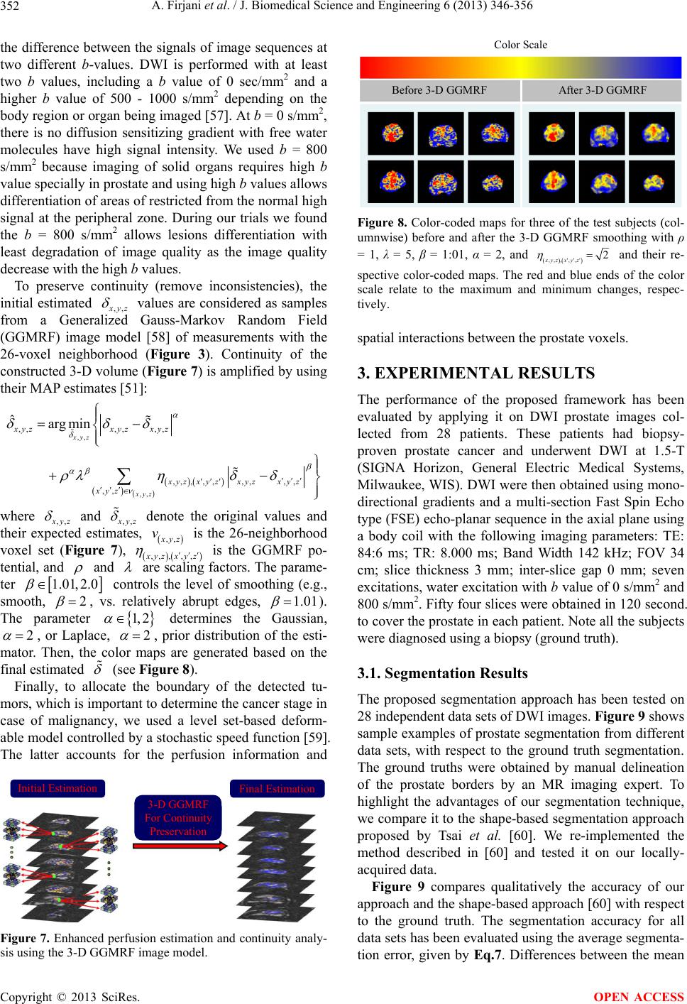

A. Firjani et al. / J. Biomedical Science and Engineering 6 (2013) 346-356 352
the difference between the signals of image sequences at
two different b-values. DWI is performed with at least
two b values, including a b value of 0 sec/mm2 and a
higher b value of 500 - 1000 s/mm2 depending on the
body region or organ being imaged [57]. At b = 0 s/mm2,
there is no diffusion sensitizing gradient with free water
molecules have high signal intensity. We used b = 800
s/mm2 because imaging of solid organs requires high b
value specially in prostate and using h igh b values allows
differentiation of areas of restricted from the normal high
signal at the peripheral zone. During our trials we found
the b = 800 s/mm2 allows lesions differentiation with
least degradation of image quality as the image quality
decrease with the high b values.
To preserve continuity (remove inconsistencies), the
initial estimated ,,
x
yz

values are considered as samples
from a Generalized Gauss-Markov Random Field
(GGMRF) image model [58] of measurements with the
26-voxel neighborhood (Figure 3). Continuity of the
constructed 3-D volu me (Figure 7) is amplified by using
their MAP estimates [51]:



,,
,,
,,,, ,,
,,, ,
,,,, ,
,,
ˆargmin
xyz
xyz
xyzxyzxyz
xyzxy z
xyzx y z
xyz






 












 






where ,,
x
yz

and ,,
x
yz denote the original values and
their expected estimates,



,,

x
yz
v is the 26-neighborhood
voxel set (Figure 7),

,,,, ,
x
yzx y z


 is the GGMRF po-
tential, and

and

are scaling factors. The parame-
ter


1.01,2
2.0
 controls the level of smoothing (e.g.,
smooth,

, vs. relatively abrupt edges, 1.01


).
The parameter determines the Gaussian,

1, 2  

2

, or Laplace, 2

, prior distribution of the esti-
mator. Then, the color maps are generated based on the
final estimated

 (see Figure 8).
Finally, to allocate the boundary of the detected tu-
mors, which is important to determine the cancer stag e in
case of malignancy, we used a level set-based deform-
able model controlled by a stochastic speed function [59].
The latter accounts for the perfusion information and
3-D GGMRF
For Continuity
Preservation
Final Estimation
Initial Estimation
Figure 7. Enhanced perfusion estimation and continuity analy-
sis using the 3-D GGMRF image model.
Color Scale
Before 3-D GGMRFAfter 3- D GGMRF
Figure 8. Color-coded maps for three of the test subjects (col-
umnwise) before and after the 3-D GGMRF smoothing with ρ
= 1, λ = 5, β = 1:01, α = 2, and
 
,, ,, ,2 xyzx y z

  and their re-
spective color-coded maps. The red and blue ends of the color
scale relate to the maximum and minimum changes, respec-
tively.
spatial interactions between the prostate voxels.
3. EXPERIMENTAL RESULTS
The performance of the proposed framework has been
evaluated by applying it on DWI prostate images col-
lected from 28 patients. These patients had biopsy-
proven prostate cancer and underwent DWI at 1.5-T
(SIGNA Horizon, General Electric Medical Systems,
Milwaukee, WIS). DWI were then obtained using mono-
directional gradients and a multi-section Fast Spin Echo
type (FSE) echo-plan ar sequence in the axial plan e using
a body coil with the following imaging parameters: TE:
84:6 ms; TR: 8.000 ms; Band Width 142 kHz; FOV 34
cm; slice thickness 3 mm; inter-slice gap 0 mm; seven
excitations, water excitatio n with b value of 0 s/mm2 and
800 s/mm2. Fifty four slices were obtained in 120 secon d.
to cover the prostate in each patient. Note all the subjects
were diagnosed using a biopsy (ground truth).
3.1. Segmentation Results
The proposed segmentation approach has been tested on
28 independent data sets of DWI images. Figure 9 shows
sample examples of prostate segmentation from different
data sets, with respect to the ground truth segmentation.
The ground truths were obtained by manual delineation
of the prostate borders by an MR imaging expert. To
highlight the advantages of our segmentation technique,
we compare it to the shape-b ased segmentation approach
proposed by Tsai et al. [60]. We re-implemented the
method described in [60] and tested it on our locally-
acquired data.
Figure 9 compares qualitatively the accuracy of our
approach and the shape-based approach [60] with respect
to the ground truth. The segmentation accuracy for all
data sets has been evaluated using the average segmenta-
tion error, given by Eq.7. Differences between the mean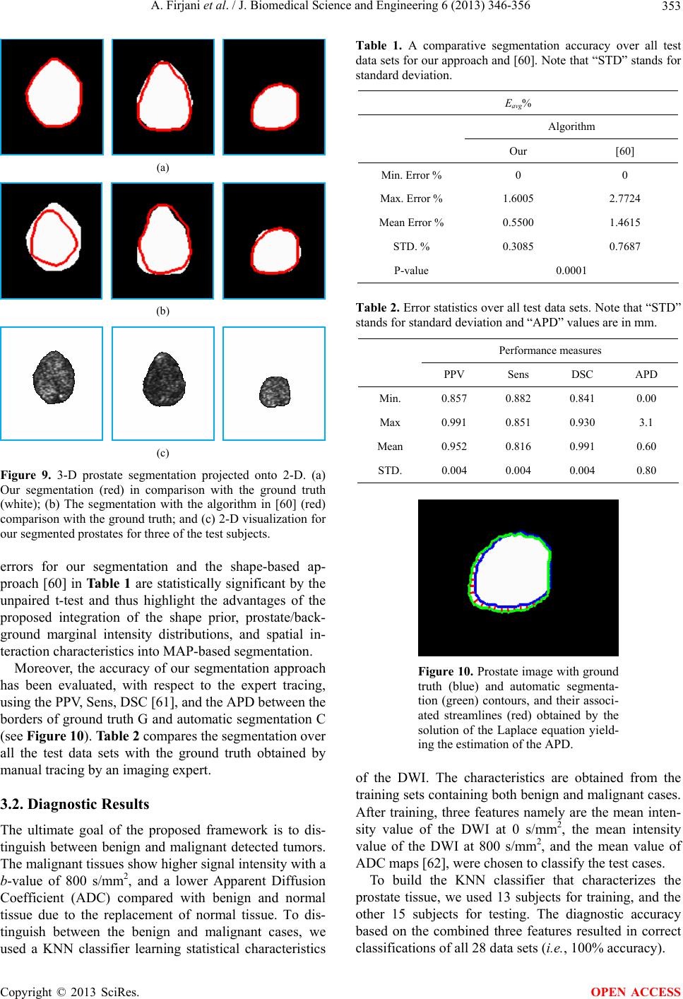

A. Firjani et al. / J. Biomedical Science and Engineering 6 (2013) 346-356 353
(a)
(b)
(c)
Figure 9. 3-D prostate segmentation projected onto 2-D. (a)
Our segmentation (red) in comparison with the ground truth
(white); (b) The segmentation with the algorithm in [60] (red)
comparison with the ground truth; and (c) 2-D visualization for
our segmented prostates for three of the test subjects.
errors for our segmentation and the shape-based ap-
proach [60] in Ta ble 1 are statistically significant by the
unpaired t-test and thus highlight the advantages of the
proposed integration of the shape prior, prostate/back-
ground marginal intensity distributions, and spatial in-
teraction characteristics into MAP-based seg mentation.
Moreover, the accuracy of our segmentation approach
has been evaluated, with respect to the expert tracing,
using the PPV, Sens, DSC [61], and the APD between the
borders of ground truth G and automatic segmentation C
(see Figure 10). Table 2 compares the segmentation over
all the test data sets with the ground truth obtained by
manual tracing by an imaging exp e rt.
3.2. Diagnostic Results
The ultimate goal of the proposed framework is to dis-
tinguish between benign and malignant detected tumors.
The malignant tissues show higher signal intensity with a
b-value of 800 s/mm2, and a lower Apparent Diffusion
Coefficient (ADC) compared with benign and normal
tissue due to the replacement of normal tissue. To dis-
tinguish between the benign and malignant cases, we
used a KNN classifier learning statistical characteristics
Table 1. A comparative segmentation accuracy over all test
data sets for our approach and [60]. Note that “STD” stands for
standard deviation.
Eavg%
Algorithm
Our [60]
Min. Error % 0 0
Max. Error % 1.6005 2.7724
Mean Error % 0.5500 1.46 15
STD. % 0.3085 0.7687
P-value 0.0001
Table 2. Error statistics over all test data sets. Note that “STD”
stands for standard deviation and “APD” values are in mm.
Performance measures
PPV Sens DSC APD
Min. 0.857 0.882 0.841 0.00
Max 0.991 0.851 0.930 3.1
Mean 0.952 0.816 0.991 0.60
STD. 0.004 0.004 0.004 0.80
Figure 10. Prostate image with ground
truth (blue) and automatic segmenta-
tion (green) contours, and their associ-
ated streamlines (red) obtained by the
solution of the Laplace equation yield-
ing the estimation of the APD.
of the DWI. The characteristics are obtained from the
training sets containing both benign and malignant cases.
After training, three features namely are the mean inten-
sity value of the DWI at 0 s/mm2, the mean intensity
value of the DWI at 800 s/mm2, and the mean value of
ADC maps [62], were chosen to classify the test cases.
To build the KNN classifier that characterizes the
prostate tissue, we used 13 subjects for training, and the
other 15 subjects for testing. The diagnostic accuracy
based on the combined three features resulted in correct
classifications of all 28 data sets (i.e., 100% accuracy).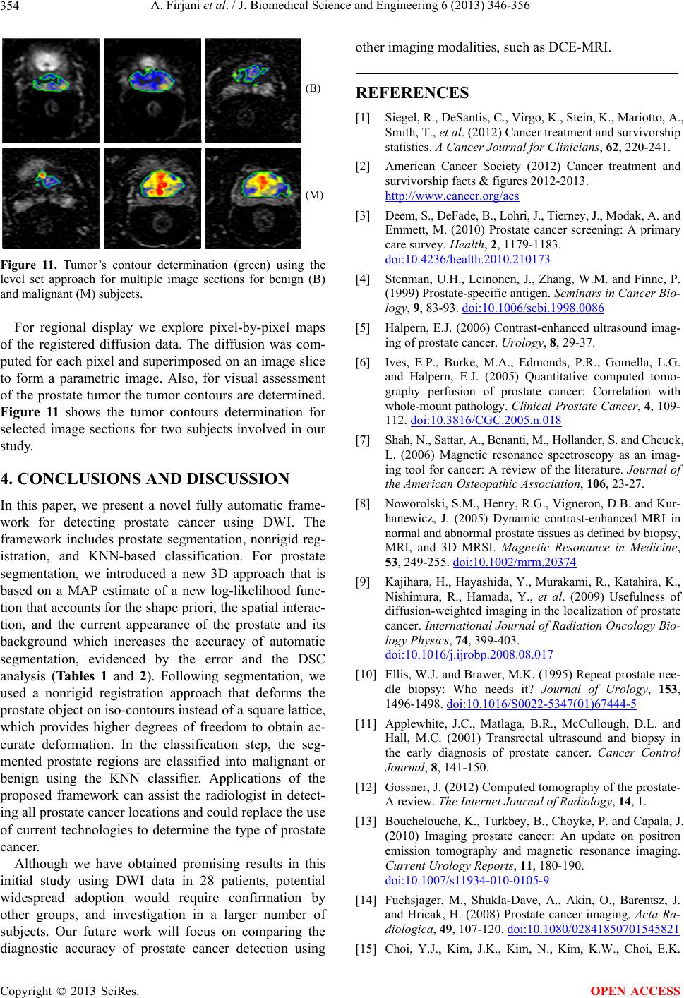

A. Firjani et al. / J. Biomedical Science and Engineering 6 (2013) 346-356 354
(B)
(M)
Figure 11. Tumor’s contour determination (green) using the
level set approach for multiple image sections for benign (B)
and malignant (M) subjects.
For regional display we explore pixel-by-pixel maps
of the registered diffusion data. The diffusion was com-
puted for each pixel and superimposed on an image slice
to form a parametric image. Also, for visual assessment
of the prostate tumor the tumor con tours are determined.
Figure 11 shows the tumor contours determination for
selected image sections for two subjects involved in our
study.
4. CONCLUSIONS AND DISCUSSION
In this paper, we present a novel fully automatic frame-
work for detecting prostate cancer using DWI. The
framework includes prostate segmentation, nonrigid reg-
istration, and KNN-based classification. For prostate
segmentation, we introduced a new 3D approach that is
based on a MAP estimate of a new log-likelihood func-
tion that accounts for the sh ape priori, the sp atial interac-
tion, and the current appearance of the prostate and its
background which increases the accuracy of automatic
segmentation, evidenced by the error and the DSC
analysis (Tables 1 and 2). Following segmentation, we
used a nonrigid registration approach that deforms the
prostate object on iso-contours instead of a square lattice,
which provides higher degrees of freedom to obtain ac-
curate deformation. In the classification step, the seg-
mented prostate regions are classified into malignant or
benign using the KNN classifier. Applications of the
proposed framework can assist the radiologist in detect-
ing all prostate cancer locations and could replace the use
of current technologies to determine the type of prostate
cancer.
Although we have obtained promising results in this
initial study using DWI data in 28 patients, potential
widespread adoption would require confirmation by
other groups, and investigation in a larger number of
subjects. Our future work will focus on comparing the
diagnostic accuracy of prostate cancer detection using
other imaging modalities, such as DCE-MRI.
REFERENCES
[1] Siegel, R., DeSantis, C., Virgo, K., Stein, K., Mariotto, A.,
Smith, T., et al. (2012) Cancer treatment and survivorship
statistics. A Cancer Journal for Clinicians, 62, 220-241.
[2] American Cancer Society (2012) Cancer treatment and
survivorship facts & figures 2012-2013.
http://www.cancer.org/acs
[3] Deem, S., DeFade, B., Lohri, J., Ti erney, J., M odak, A. and
Emmett, M. (2010) Prostate cancer screening: A primary
care survey. Health, 2, 1179-1183.
doi:10.4236/health.2010.210173
[4] Stenman, U.H., Leinonen, J., Zhang, W.M. and Finne, P.
(1999) Prostate-specific antigen. Seminars in Cancer Bio-
logy, 9, 83-93. doi:10.1006/scbi.1998.0086
[5] Halpern, E.J. (2006) Contrast-enhanced ultrasound imag-
ing of prostate cancer. Urology, 8, 29-37.
[6] Ives, E.P., Burke, M.A., Edmonds, P.R., Gomella, L.G.
and Halpern, E.J. (2005) Quantitative computed tomo-
graphy perfusion of prostate cancer: Correlation with
whole-mount pat hology. Clinical Prostate Cancer, 4, 109-
112. doi:10.3816/CGC.2005.n.018
[7] Shah, N., Sattar, A., Benanti, M., Hollander, S. and Cheuck,
L. (2006) Magnetic resonance spectroscopy as an imag-
ing tool for cancer: A review of the literature. Journal of
the American Osteopathic Association, 106, 23-27.
[8] Noworolski, S.M., Henry , R.G., Vigneron, D.B. and Kur-
hanewicz, J. (2005) Dynamic contrast-enhanced MRI in
normal and abnormal prostate tissues as defined by b io p sy ,
MRI, and 3D MRSI. Magnetic Resonance in Medicine,
53, 249-255. doi:10.1002/mrm.20374
[9] Kajihara, H., Hayashida, Y., Murakami, R., Katahira, K.,
Nishimura, R., Hamada, Y., et al. (2009) Usefulness of
diffusion-weighted imaging in the localization of prostate
cancer. International Journal of Radiation Oncology Bio-
logy Physics, 74, 399-403.
doi:10.1016/j.ijrobp.2008.08.017
[10] Ellis, W.J. and Brawer, M.K. (1995) Repeat prostate nee-
dle biopsy: Who needs it? Journal of Urology, 153,
1496-1498. doi:10.1016/S0022-5347(01)67444-5
[11] Applewhite, J.C., Matlaga, B.R., McCullough, D.L. and
Hall, M.C. (2001) Transrectal ultrasound and biopsy in
the early diagnosis of prostate cancer. Cancer Control
Journal, 8, 141-150.
[12] Gossner, J. (2012) Computed tomography of the prostate-
A review. The Internet Journal of Radiology, 14, 1.
[13] Bouchelouche, K., Turkbey, B., Choyke, P. and Capala, J.
(2010) Imaging prostate cancer: An update on positron
emission tomography and magnetic resonance imaging.
Current Urology Reports, 11, 180-190.
doi:10.1007/s11934-010-0105-9
[14] Fuchsjager, M., Shukla-Dave, A., Akin, O., Barentsz, J.
and Hricak, H. (2008) Prostate cancer imaging. Acta Ra-
diologica, 49, 107-120. doi:10.1080/02841850701545821
[15] Choi, Y.J., Kim, J.K., Kim, N., Kim, K.W., Choi, E.K.

A. Firjani et al. / J. Biomedical Science and Engineering 6 (2013) 346-356 355
and Cho, K.S. (2007) Functional MR imaging of prostate
cancer. RadioGraphics, 27, 63-75.
doi:10.1148/rg.271065078
[16] Zakian, K.L., Eberhardt, S., Hricak, H., Shukla-Dave, A.,
Kleinman, S., Muruganandham, M., et al. (2003) Tran-
sition zone prostate cancer: Metabolic characteristics at
1H MR spectroscopic imaging-initial results. Radiology,
229, 241-247. doi:10.1148/radiol.2291021383
[17] Punwani, S., Emberton, M., Walkden, M., Sohaib, A.,
Freeman, A., Ahmed, H., et al. (2012) Prostatic cancer
surveillance following whole-gland high-intensity focused
ultrasound: Comparison of MRI and prostate-specific an-
tigen for detection of residual or recurrent disease. British
Journal of Radiology, 85, 720-728.
doi:10.1259/bjr/61380797
[18] Bhave, G., Lewis, Julia, B. and Chang, S. (2008) Asso-
ciation of gadolinium based magnetic resonance imaging
contrast agents and nephrogenic systemic fibrosis. Jour-
nal of Urology, 180, 830-835.
doi:10.1016/j.juro.2008.05.005
[19] Yu, K.K. and Hricak, H. (2000) Imaging prostate cancer.
Radiologic Clinics of North America, 38, 59-85.
doi:10.1016/S0033-8389(05)70150-0
[20] Ikonen, S., Karkkainen, P., Kivisaari, L., Salo, J.O., Taari,
K., Vehmas, T., et al. (2001) Endorectal magnetic re-so-
nance imaging of prostatic cancer: Comparison between
fat-suppressed T2-weighted fast spin echo and three-di-
mensional dual-echo, steady-state sequences. European
Radiology, 11, 236-241. doi:10.1007/s003300000598
[21] Shimofusa, R., Fujimoto, H., Akamata, H., Motoori, K.,
Yamamoto, S. , Ueda, T ., et al. (2005) Diffusion-weighted
imaging of prostate cancer. Journal of Computer Assisted
Tomography, 29, 149-153.
doi:10.1097/01.rct.0000156396.13522.f2
[22] Hacklander, T., Scharwachter, C., Golz, R. and Mertens,
H. (2006) Value of diffusion-weighted imaging for diag-
nosing vertebral metastases due to prostate cancer in
comparison to other primary tumors. Rofo, 178, 416-424.
[23] Yoshimitsu, K., Kiyoshima, K., Irie, H., Tajima, T.,
Asayama, Y., Hirakawa, M., et al. (2008) Usefulness of
apparent diffusion coefficient map in diagnosing prostate
carcinoma: Correlation with stepwise histopathology. Jour-
nal of Magnetic Resonance Imaging, 27, 132-139.
doi:10.1002/jmri.21181
[24] Lim, H.K., Kim, J.K., Kim, K.A. and Cho, K.S. (2009)
Prostate cancer: Apparent diffusion coefficient map with
T2-weighted images for detection a multireader study.
Radiology, 250, 145-151. doi:10.1148/radiol.2501080207
[25] Haider, M.A., van der Kwast, T.H., Tanguay, J., Evans,
A.J., Hashmi, A.T., Lockwood, G., et al. (2007) Com-
bined T2-weighted and diffusion-weighted MRI for loca-
lization of prostate cancer. American Journal of Roent-
genology, 189, 323-328. doi:10.2214/AJR.07.2211
[26] Padhani, A.R., Liu, G., Koh, D.M., Chenevert, T.L.,
Thoeny, H.C., Takahara, T., et al. (2009) Diffusion-
weighted magnetic resonance imaging as a cancer bio-
marker: Consensus and recommendations. Neoplasia, 11,
102-125.
[27] Kitajima, K., Kaji, Y., Fukabori, Y., Yoshida, K., Suga-
numa, N. and Sugimura, K. (2010) Prostate cancer detec-
tion with 3T MRI: Comparison of diffusion-weighted
imaging and dynamic contrast-enhanced MRI in com-
bination with T2-weighted imaging. Journal of Magnetic
Resonance Imaging, 31, 625-631. doi:10.1002/jmri.22075
[28] Iwazawa, J., Mitani, T., Sassa, S. and Ohue, S. (2011)
Prostate cancer detection with MRI: Is dynamic contrast-
enhanced imaging necessary in addition to diffusion-
weighted imaging? Diagnostic and Interventional Radiology,
17, 243-248.
[29] Kim, C.K., Park, B.K. and Lee, H.M. (2009) Prediction
of locally recurrent prostate cancer after radiation therapy:
Incremental value of 3T diffusion-weighted MRI. Journal
of Magnetic Resonance Imaging, 29, 391-397.
doi:10.1002/jmri.21645
[30] Tan, C.H., Wang, J. and Kundra, V. (2011) Diffusion
weighted imaging in prostate cancer. European Radiology,
21, 593-603. doi:10.1007/s00330-010-1960-y
[31] Chan, I., Wells, III, W., Mulkern, R.V., Haker, S., Zhang,
J., Zou, K.H., et al. (2003) Detection of prostate cancer
by integration of line-scan diffusion, T2-mapping and
T2-weighted magnetic resonance imaging; a multichannel
statistical classifier. Journal of Medical Physics, 30, 2390-
2398. doi:10.1118/1.1593633
[32] Huisman, H., Vos, P., Litjens, G., Hambrock, T. and
Barentsz, J. (2010) Computer aided detection of prostate
cancer using t2w, DWI and DCE-MRI: Methods and
clinic al ap plica tio ns. Proceedings of International Workshop,
Held in Conjunction with MICCAI 2010, Beijing, 20-24
September 2010, 4-14.
[33] Frangi, A.F., Niessen, W.J. , Vincken, K.L. and Viergever,
M.A. (1998) Multiscale vessel enhancement filtering.
Proceedings of the 1st Annual International Conference
of the MICCA, Cambridge, 11-13 October 1998, 130-137.
[34] Viswanath, S., Bloch, B.N., Genega, E., Rofsky, N., Len-
kinski, R., Chappelow, J., et al. (2008) A comprehensive
segmentation, registration, and cancer detection scheme
on 3 Tesla in vivo prostate DCE-MRI. Medical Image
Computing and Computer-Assisted Intervention, 11, 662-
669.
[35] Langer, Deanna, L., van der Kwast Theodorus, H., Evans,
Andrew, J., et al. (2009) Prostate cancer detection with
multi-parametric MRI: Logistic regression analysis of
quantitative T2, diffusion-weighted imaging, and dynamic
contrast-enhanced MRI. Journal of Magnetic Resonance
Imaging, 30, 327-334. doi:10.1002/jmri.21824
[36] Villeirs, G.M., L Verstraete, K., De Neve, W.J. and De
Meerleer, G.O. (2005) Magnetic resonance imaging ana-
tomy of the prostate and periprostatic area: A guide for
radiotherapists. Radiotherapy and Oncology, 76, 99-106.
doi:10.1016/j.radonc.2005.06.015
[37] Zhan, Y. and Shen, D. (2003) Automated segmentation of
3D US prostate images using statistical texture-based
matching method. Proceedings of the 6th Annual Interna-
tional Conference of the MICCA, Montreal, 15-18 Nove-
mber 2003, 2878, 688-696.
[38] Lixin, G., Pathak, S.D., Haynor, D.R., Cho, P.S. and Kim,
Y. (2004) Parametric shape modeling using deformable
superellipses for prostate segmentation. IEEE Transac-

A. Firjani et al. / J. Biomedical Science and Engineering 6 (2013) 346-356 356
tions on Medical Imaging, 23, 340-349.
doi:10.1109/TMI.2004.824237
[39] Zwiggelaar, R., Zhu, Y. and Williams, S. (2003) Semi-
automatic segmentation of the prostate. Pattern Recog-
nition and Image Analysis, 2652, 1108-1116.
doi:10.1007/978-3-540-44871-6_128
[40] Zhu, Y., Williams, S. and Zwiggelaar, R. (2004) Segmen-
tation of volumetric prostate MRI data using hybrid
2d+3d shape modeling. Medical Image Understanding and
Analysis, 61-64.
[41] Toth, R., Tiwari, P., Rosen, M., Kalyanpur, A., P ung avk ar,
S. and Madabhushi, A. (2008) A multi-modal prostate
segmentation scheme by combining spectral clustering
and active shape models. Proceedings of the International
Society of Optics and Photonic, San Jo se, 691 44 S- 6 9144S.
[42] Klein, S., van der Heide, U.A., Raaymakers, B.W., Kot te,
A.N.T.J., Staring, M. and Pluim, J.P.W. (2007) Segmen-
tation of the prostate in MR images by atlas matching.
Proceedings of the 4th Annual IEEE International Sym-
posium on Biomedical Imaging: From Nano to Macro
(ISBI), Washington DC, 12-15 April 2007, 1300-1303.
[43] Vikal, S., Haker, S., Tempany, C. and Fichtinger, G. (2009)
Prostate contouring in MRI guided biopsy. Proceedings
of the International Society of Optics and Photonics, 7259,
72594A.
[44] Martin, S., Troccaz, J. and Daanenc, V. (2010) Auto-
mated segmentation of the prostate in 3D MR images us-
ing a probabilistic atlas and a spatially constrained de-
formable model. Journal of Medical Physics, 37, 1579-
1590. doi:10.1118/1.3315367
[45] Hambrock, T., Somford, D.M., Hoeks, C., Bouwense, S.
A., Huisman, H., Yakar, D., et al. (2010) Magnetic re-
sonance imaging guided prostate biopsy in men with re-
peat negative biopsies and increased prostate specific an-
tigen. Journal of Urology, 183, 520-527.
doi:10.1016/j.juro.2009.10.022
[46] Firjani, A., Khalifa, F., Elnakib, A., Gimel’farb, G., El-
Ghar, M.A., Elmaghraby, A. and El-Baz, A. (2011) 3D
automatic approach for precise segmentation of the pr ost ate
from diffusion-weighted magnetic resonance imaging.
Proceedings of 18th Annual IEEE International Conference
on Image Processing (ICIP), Brussels, 11-14 September
2011, 2285-2288.
[47] Firjani, A., Khalifa, F., Elnakib, A., Gimel’farb, G., El-
Ghar, M.A., Elmaghraby, A. and El-Baz, A. (2012) A
novel image-based approach f or early detection of p ro sta te
cancer. Proceedings of 19th Annual IEEE International
Conference on Image Processing (ICIP), Orlando, 30 Se p-
tember-3 October 2012, 2849-2852.
[48] Firjani, A., Elnakib, A., Khalifa, F., Gimel’farb, G., El-
Ghar, M.A., Elmaghraby, A. and El-Baz, A. (2011) A
new 3D automatic segmentation framework for accurate
extraction of prostate from diffusion imaging. Proceed-
ings of 3rd Annual Biomedical Sciences and Engineering
Conference (BSEC), Knoxville, 15-17 March 2011, 1-4.
[49] El-Baz, A., Gimel’farb, G., Falk, R., Holland, T. and
Shaffer, T. (2008) A new stochastic framework for accurate
lung segmentation. Proceedings of the 11th Annual Inter-
national Conference of the MICCA, New York, 6-10 Sep-
tember 2008, 322-330.
[50] El-Baz, A., Elnakib, A., Khalifa, F., Abou El-Ghar, M.,
McClure, P., Soliman, A. an d Gimel’farb, G. (2012) Pre-
cise segmentation of 3-D magnetic resonance angio-
graphy. IEEE Transactions on Biomedical Engineering, 7,
2019-2029. doi:10.1109/TBME.2012.2196434
[51] El-Baz, A. and Gimel’farb, G. (2007) EM based approxi-
mation of empirical distributions with linear combinations
of discrete Gaussians. Proceedings of 14th Annual IEEE
International Conference on Image Processing (ICIP),
San Antonio, 16-19 September 2007, 4, 373-376.
[52] Farag, A.A., El-Baz, A. and Gimel’farb, G. (2006) P rec ise
segmentation of multi-modal images. IEEE Transactions
on Image Processing, 15, 952-968.
doi:10.1109/TIP.2005.863949
[53] El-Baz, A. (2006) Novel stochastic models for medical
image analysis. Ph.D. Thesis, University of Louisville,
Louisville.
[54] Viola, P. and Wells, W.M. (1997) Alignment by maxi-
mization of mutual information. International Journal of
Computer Vision, 24, 137-154.
doi:10.1023/A:1007958904918
[55] Besag, J. (1986) On the statistical-analysis of dirty pic-
tures. Journal of the Royal Statistical Society Series B-
Methodological, 48, 259-302.
[56] Khalifa, F., El-Baz, A., Gimel’farb, G. and Abu El-Ghar.
M. (2010) Non-invasive image-based approach for early
detection of acute renal rejection. Proceedings of the 13th
Annual International Conference of the MICCA, Beijing,
20-24 September 2010, 1, 10-18.
[57] Patterson, D.M., Padhani, A.R. and Collins, D.J. (2008)
Technology insight: Water diffusion MRI—A potential
new biomarker of response to cancer therapy. Nature Cli-
nical Practice Oncology, 5, 220-233.
doi:10.1038/ncponc1073
[58] Bouman, C. and Sauer, K. (1993) A generalized Gaussian
image model for edge-preserving MAP estimation. IEEE
Transactions on Image Processing, 2, 296-310.
doi:10.1109/83.236536
[59] Khalifa, F., Beache, G.M., Gimelrfarb, G., Giridharan,
G.A. and El-Baz, A. (2012) Accurate automatic analysis
of cardiac cine images. IEEE Transactions on Biomedical
Engineering, 59, 445-455.
doi:10.1109/TBME.2011.2174235
[60] Tsai, A., Yezzi, Jr., A., Wells, W., Tempany, C., Tucker,
D., Fan, A., et al. (2003) A shape-based approach to the
segmentation of medical imagery using level sets. IEEE
Transactions on Medical Imaging, 22, 137-154.
doi:10.1109/TMI.2002.808355
[61] Dice, L.R. (1945) Measures of the amount of ecologic
association between species. Ecology, 26, 297-302.
doi:10.2307/1932409
[62] Walker-Samuel, S., Orton, M., Boult, J.K. and Robinson,
S.P. (2011) Improving apparent diffusion coefficient esti-
mates and elucidating tu mor heterogeneity using Baye sian
adaptive smoothing. Magnetic Resonance in Medicine, 65,
438-447. doi:10.1002/mrm.22572