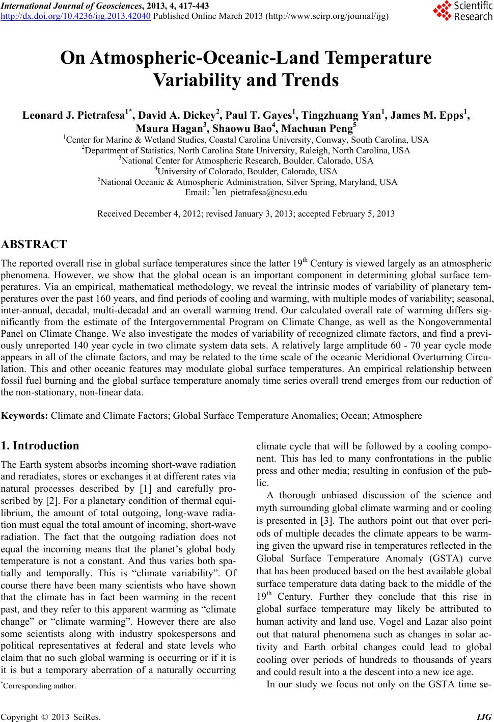
 International Journal of Geosciences, 2013, 4, 417-443 http://dx.doi.org/10.4236/ijg.2013.42040 Published Online March 2013 (http://www.scirp.org/journal/ijg) On Atmospheric-Oceanic-Land Temperature Variability and Trends Leonard J. Pietrafesa1*, David A. Dickey2, Paul T. Gayes1, Tingzhuang Yan1, James M. Epps1, Maura Hagan3, Shaowu Bao4, Machuan Peng5 1Center for Marine & Wetland Studies, Coastal Carolina University, Conway, South Carolina, USA 2Department of Statistics, North Carolina State University, Raleigh, North Carolina, USA 3National Center for Atmospheric Research, Boulder, Calorado, USA 4University of Colorado, Boulder, Calorado, USA 5 National Oceanic & Atmospheric Administration, Silver Spring, Maryland, USA Email: *len_pietrafesa@ncsu.edu Received December 4, 2012; revised January 3, 2013; accepted February 5, 2013 ABSTRACT The reported overall rise in global surface temperatures since the latter 19th Century is viewed largely as an atmospheric phenomena. However, we show that the global ocean is an important component in determining global surface tem- peratures. Via an empirical, mathematical methodology, we reveal the intrinsic modes of variability of planetary tem- peratures over the past 160 years, and find periods of cooling and warming, with multiple modes of variability; seasonal, inter-annual, decadal, multi-decadal and an overall warming trend. Our calculated overall rate of warming differs sig- nificantly from the estimate of the Intergovernmental Program on Climate Change, as well as the Nongovernmental Panel on Climate Change. We also investigate the modes of variability of recognized climate factors, and find a previ- ously unreported 140 year cycle in two climate system data sets. A relatively large amplitude 60 - 70 year cycle mode appears in all of the climate factors, and may be related to the time scale of the oceanic Meridional Overturning Circu- lation. This and other oceanic features may modulate global surface temperatures. An empirical relationship between fossil fuel burning and the global surface temperature anomaly time series overall trend emerges from our reduction of the non-stationary, non-linear data. Keywords: Climate and Climate Factors; Global Surface Temperature Anomalies; Ocean; Atmosphere 1. Introduction The Earth system absorbs incoming short-wave radiation and reradiates, stores or exchanges it at different rates via natural processes described by [1] and carefully pro- scribed by [2]. For a planetary condition of thermal equi- librium, the amount of total outgoing, long-wave radia- tion must equal the total amount of incoming, short-wave radiation. The fact that the outgoing radiation does not equal the incoming means that the planet’s global body temperature is not a constant. And thus varies both spa- tially and temporally. This is “climate variability”. Of course there have been many scientists who have shown that the climate has in fact been warming in the recent past, and they refer to this apparent warming as “climate change” or “climate warming”. However there are also some scientists along with industry spokespersons and political representatives at federal and state levels who claim that no such global warming is occurring or if it is it is but a temporary aberration of a naturally occurring climate cycle that will be followed by a cooling compo- nent. This has led to many confrontations in the public press and other media; resulting in confusion of the pub- lic. A thorough unbiased discussion of the science and myth surrounding global climate warming and or cooling is presented in [3]. The authors point out that over peri- ods of multiple decades the climate appears to be warm- ing given the upward rise in temperatures reflected in the Global Surface Temperature Anomaly (GSTA) curve that has been produced based on the best available global surface temperature data dating back to the middle of the 19th Century. Further they conclude that this rise in global surface temperature may likely be attributed to human activity and land use. Vogel and Lazar also point out that natural phenomena such as changes in solar ac- tivity and Earth orbital changes could lead to global cooling over periods of hundreds to thousands of years and could result into a the descent into a new ice age. In our study we focus not only on the GSTA time se- *Corresponding author. C opyright © 2013 SciRes. IJG 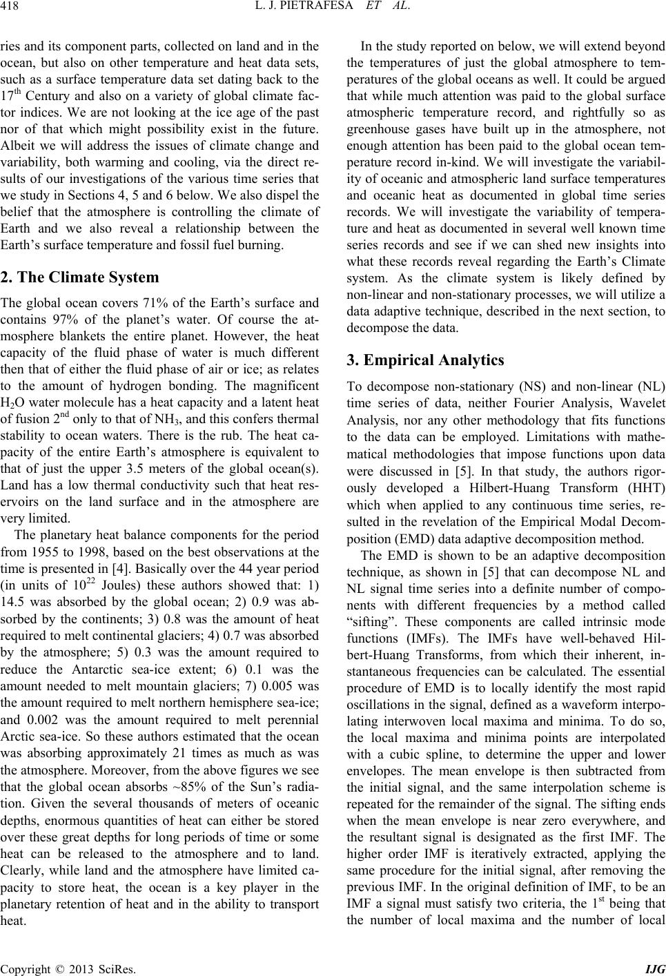 L. J. PIETRAFESA ET AL. 418 ries and its component parts, collected on land and in the ocean, but also on other temperature and heat data sets, such as a surface temperature data set dating back to the 17th Century and also on a variety of global climate fac- tor indices. We are not looking at the ice age of the past nor of that which might possibility exist in the future. Albeit we will address the issues of climate change and variability, both warming and cooling, via the direct re- sults of our investigations of the various time series that we study in Sections 4, 5 and 6 below. We also dispel the belief that the atmosphere is controlling the climate of Earth and we also reveal a relationship between the Earth’s surface temperature and fossil fuel burning. 2. The Climate System The global ocean covers 71% of the Earth’s surface and contains 97% of the planet’s water. Of course the at- mosphere blankets the entire planet. However, the heat capacity of the fluid phase of water is much different then that of either the fluid phase of air or ice; as relates to the amount of hydrogen bonding. The magnificent H2O water molecule has a heat capacity and a latent heat of fusion 2nd only to that of NH3, and this confers thermal stability to ocean waters. There is the rub. The heat ca- pacity of the entire Earth’s atmosphere is equivalent to that of just the upper 3.5 meters of the global ocean(s). Land has a low thermal conductivity such that heat res- ervoirs on the land surface and in the atmosphere are very limited. The planetary heat balance components for the period from 1955 to 1998, based on the best observations at the time is presented in [4]. Basically over the 44 year period (in units of 1022 Joules) these authors showed that: 1) 14.5 was absorbed by the global ocean; 2) 0.9 was ab- sorbed by the continents; 3) 0.8 was the amount of heat required to melt continental glaciers; 4) 0.7 was absorbed by the atmosphere; 5) 0.3 was the amount required to reduce the Antarctic sea-ice extent; 6) 0.1 was the amount needed to melt mountain glaciers; 7) 0.005 was the amount required to melt northern hemisphere sea-ice; and 0.002 was the amount required to melt perennial Arctic sea-ice. So these authors estimated that the ocean was absorbing approximately 21 times as much as was the atmosphere. Moreover, from the above figures we see that the global ocean absorbs ~85% of the Sun’s radia- tion. Given the several thousands of meters of oceanic depths, enormous quantities of heat can either be stored over these great depths for long periods of time or some heat can be released to the atmosphere and to land. Clearly, while land and the atmosphere have limited ca- pacity to store heat, the ocean is a key player in the planetary retention of heat and in the ability to transport heat. In the study reported on below, we will extend beyond the temperatures of just the global atmosphere to tem- peratures of the global oceans as well. It could be argued that while much attention was paid to the global surface atmospheric temperature record, and rightfully so as greenhouse gases have built up in the atmosphere, not enough attention has been paid to the global ocean tem- perature record in-kind. We will investigate the variabil- ity of oceanic and atmospheric land surface temperatures and oceanic heat as documented in global time series records. We will investigate the variability of tempera- ture and heat as documented in several well known time series records and see if we can shed new insights into what these records reveal regarding the Earth’s Climate system. As the climate system is likely defined by non-linear and non-stationary processes, we will utilize a data adaptive technique, described in the next section, to decompose the data. 3. Empirical Analytics To decompose non-stationary (NS) and non-linear (NL) time series of data, neither Fourier Analysis, Wavelet Analysis, nor any other methodology that fits functions to the data can be employed. Limitations with mathe- matical methodologies that impose functions upon data were discussed in [5]. In that study, the authors rigor- ously developed a Hilbert-Huang Transform (HHT) which when applied to any continuous time series, re- sulted in the revelation of the Empirical Modal Decom- position (EMD) data adaptive decomposition method. The EMD is shown to be an adaptive decomposition technique, as shown in [5] that can decompose NL and NL signal time series into a definite number of compo- nents with different frequencies by a method called “sifting”. These components are called intrinsic mode functions (IMFs). The IMFs have well-behaved Hil- bert-Huang Transforms, from which their inherent, in- stantaneous frequencies can be calculated. The essential procedure of EMD is to locally identify the most rapid oscillations in the signal, defined as a waveform interpo- lating interwoven local maxima and minima. To do so, the local maxima and minima points are interpolated with a cubic spline, to determine the upper and lower envelopes. The mean envelope is then subtracted from the initial signal, and the same interpolation scheme is repeated for the remainder of the signal. The sifting ends when the mean envelope is near zero everywhere, and the resultant signal is designated as the first IMF. The higher order IMF is iteratively extracted, applying the same procedure for the initial signal, after removing the previous IMF. In the original definition of IMF, to be an IMF a signal must satisfy two criteria, the 1st being that the number of local maxima and the number of local Copyright © 2013 SciRes. IJG 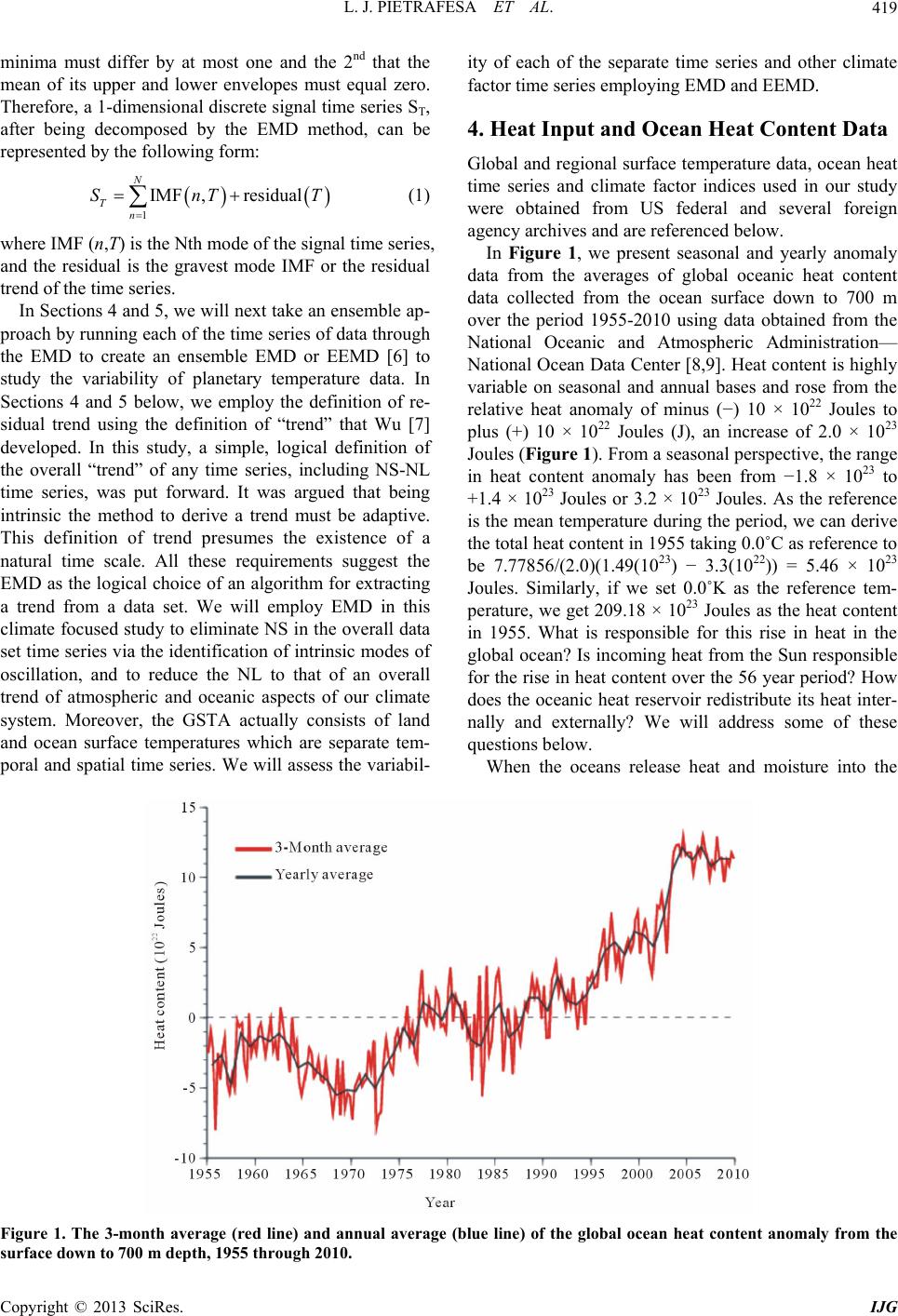 L. J. PIETRAFESA ET AL. Copyright © 2013 SciRes. IJG 419 T minima must differ by at most one and the 2nd that the mean of its upper and lower envelopes must equal zero. Therefore, a 1-dimensional discrete signal time series ST, after being decomposed by the EMD method, can be represented by the following form: ity of each of the separate time series and other climate factor time series employing EMD and EEMD. 4. Heat Input and Ocean Heat Content Data Global and regional surface temperature data, ocean heat time series and climate factor indices used in our study were obtained from US federal and several foreign agency archives and are referenced below. 1 IMF ,residual N Tn SnT (1) where IMF (n,T) is the Nth mode of the signal time series, and the residual is the gravest mode IMF or the residual trend of the time series. In Figure 1, we present seasonal and yearly anomaly data from the averages of global oceanic heat content data collected from the ocean surface down to 700 m over the period 1955-2010 using data obtained from the National Oceanic and Atmospheric Administration— National Ocean Data Center [8,9]. Heat content is highly variable on seasonal and annual bases and rose from the relative heat anomaly of minus (−) 10 × 1022 Joules to plus (+) 10 × 1022 Joules (J), an increase of 2.0 × 10²³ Joules (Figure 1). From a seasonal perspective, the range in heat content anomaly has been from −1.8 × 10²³ to +1.4 × 10²³ Joules or 3.2 × 10²³ Joules. As the reference is the mean temperature during the period, we can derive the total heat content in 1955 taking 0.0˚C as reference to be 7.77856/(2.0)(1.49(1023) − 3.3(1022)) = 5.46 × 10²³ Joules. Similarly, if we set 0.0˚K as the reference tem- perature, we get 209.18 × 10²³ Joules as the heat content in 1955. What is responsible for this rise in heat in the global ocean? Is incoming heat from the Sun responsible for the rise in heat content over the 56 year period? How does the oceanic heat reservoir redistribute its heat inter- nally and externally? We will address some of these questions below. In Sections 4 and 5, we will next take an ensemble ap- proach by running each of the time series of data through the EMD to create an ensemble EMD or EEMD [6] to study the variability of planetary temperature data. In Sections 4 and 5 below, we employ the definition of re- sidual trend using the definition of “trend” that Wu [7] developed. In this study, a simple, logical definition of the overall “trend” of any time series, including NS-NL time series, was put forward. It was argued that being intrinsic the method to derive a trend must be adaptive. This definition of trend presumes the existence of a natural time scale. All these requirements suggest the EMD as the logical choice of an algorithm for extracting a trend from a data set. We will employ EMD in this climate focused study to eliminate NS in the overall data set time series via the identification of intrinsic modes of oscillation, and to reduce the NL to that of an overall trend of atmospheric and oceanic aspects of our climate system. Moreover, the GSTA actually consists of land and ocean surface temperatures which are separate tem- poral and spatial time series. We will assess the variabil- When the oceans release heat and moisture into the Figure 1. The 3-month average (red line) and annual average (blue line) of the global ocean heat content anomaly from the surface down to 700 m depth, 1955 through 2010.  L. J. PIETRAFESA ET AL. 420 atmosphere, climate factors and conditions can be altered and atmospheric eddies, aka “atmospheric storms”, can form. Heat and thus energy are then redistributed by the atmosphere, principally from the equatorial zone to the Polar zones. Likewise oceanic western boundary currents move heat from the Equatorial to the Polar Regions and large scale vertical plane ocean circulations such as the southward flowing deep branch of the Atlantic Merid- ional Overturning Circulation (the MOC) which moves cold, saline water from the Poles towards the Equator, thus having the net effect of increasing the meridional heat distribution in a poleward direction. The MOC has been referred to as the Themohaline Circulation (THC) of the ocean, that is the part of the circulation controlled by temperature and salinity variations, but the two are synonymous [10]. According to these authors, the MOC is the zonal integral of the meridional velocity while the THC is a mechanism involved in the overturning. This begs the question: What does the overall heat content record actually mean in terms of any associated increases or falls in the surface temperature of the global ocean? In Figure 2, we see the EEMD of the Global Heat Content 3-monthly averaged time series over the period of 1955-2009. There are 7 intrinsic modes. Modes shown are C1, 3 - 6 monthly, C2 annual to inter-annual, C3 a 2 - 4 year cycle, C4, a 7 - 8 year cycle, C5, an approximately 20 year cycle, and C6, ~30 year cycle and the gravest mode, an overall trend which has risen significantly over the length of the record. Figure 3 is a Sunspot activity time series obtained from the National Center for Atmospheric Research (NCAR) and shows that solar activity is highly tempo- rally variable, with the near-11 year cycle very visually prominent, about a relatively flat trend. The oceans and atmosphere could be responding to Sunspot occurrences. From the record, Sunspot activity from the present back to the middle-19th Century shows 9 modes, with Mode 9, a flat trend. Mode 8 is a nearly record length oscillation of ~155 years and Mode 7 is of the order of 55 - 60 years. Mode 6 is ~22 years and Mode 5 is centered about 11 Figure 2. EEMD of the 3 month average global ocean heat content time series. Copyright © 2013 SciRes. IJG 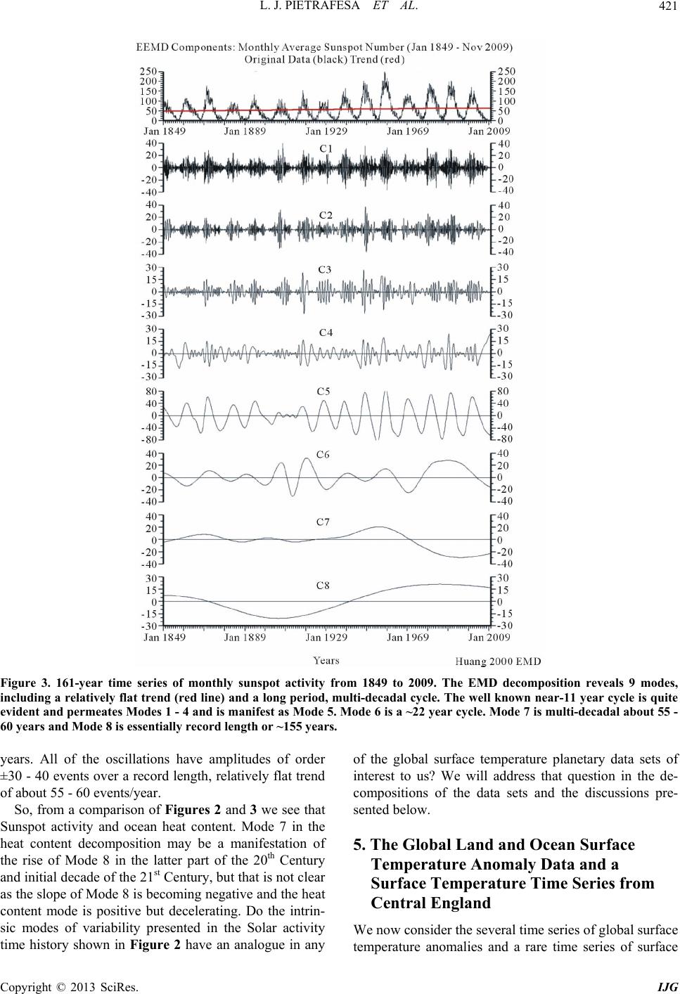 L. J. PIETRAFESA ET AL. 421 Figure 3. 161-year time series of monthly sunspot activity from 1849 to 2009. The EMD decomposition reveals 9 modes, including a relatively flat trend (red line) and a long period, multi-decadal cycle. The well known near-11 year cycle is quite evident and permeates Modes 1 - 4 and is manifest as Mode 5. Mode 6 is a ~22 year cycle. Mode 7 is multi-decadal about 55 - 60 years and Mode 8 is essentially record length or ~155 years. years. All of the oscillations have amplitudes of order ±30 - 40 events over a record length, relatively flat trend of about 55 - 60 events/year. So, from a comparison of Figures 2 and 3 we see that Sunspot activity and ocean heat content. Mode 7 in the heat content decomposition may be a manifestation of the rise of Mode 8 in the latter part of the 20th Century and initial decade of the 21st Century, but that is not clear as the slope of Mode 8 is becoming negative and the heat content mode is positive but decelerating. Do the intrin- sic modes of variability presented in the Solar activity time history shown in Figure 2 have an analogue in any of the global surface temperature planetary data sets of interest to us? We will address that question in the de- compositions of the data sets and the discussions pre- sented below. 5. The Global Land and Ocean Surface Temperature Anomaly Data and a Surface Temperature Time Series from Central England We now consider the several time series of global surface temperature anomalies and a rare time series of surface Copyright © 2013 SciRes. IJG  L. J. PIETRAFESA ET AL. 422 temperatures taken in Central England. These four data sets were obtained from the Hadley Cru website for the Southern and Northern Hemispheres (http://www.cru.uea.ac.uk/cru/info/warming/), the com- bined Global Surface Temperature Anomaly (GSTA) record and the data set from England. In Figure 4 we present the time series showing the combined global land and marine surface temperature record from 1850 to 2009. This time series is continu- ously compiled jointly by the Climatic Research Unit and the UK Meteorology Office, Hadley Centre. In Figure 5, the IPCC (2007) representation of the GSTA is presented. Superimposed on the temperature curve of the rate of planetary surface warming are the IPCC estimates of the secular rates of warming range from 0.045˚C (the 150 year red line) to 0.74˚C (the 100 year blue line) to 0.128˚C (the 50 year pink line) to 0.177˚C (the 25 year yellow line). It is of note that the much quoted estimate of ~2˚C of projected warming over the 21st Century is derived from the slope of the yellow line. However, the question arises, is this legitimate to estimate a rate of change of what is clearly a non-sta- tionary time series? Let us reconsider the time series of the GSTA (Figure 4(c)), but this time we will apply EEMD to decompose the total ocean-land-atmosphere time series (Figure 6(a)), of ocean surface temperatures only (Figure 6(b)) and the land atmospheric temperatures only (Figure 6(c)). We see that there are 9 modes of variability in each time se- ries with the 9th mode being the overall trend of the data; shown as the red lines. Remarkably, the separate ocean and land time series, which are collected totally inde- Figure 4. The Hadley Center CRU semi-global and goobal surface temperature anomaly time series from 1850-2011. Top panel: The blue shaded area represents the time series of annual values for the Northern Hemisphere and the black line is the running five-year average; Middle panel: The blue shaded area represents the time series of annual values for the Southern Hemisphere and the black line is the running five-year average; Bottom panel: The blue shaded area represents the time series of annual values for the averages between the Northern and Southern Hemispheres and the black line is the running five-year average. Figure 5. The IPCC estimates of the rate of warming using straight line estimates. The IPCC secular rates of warming range from 0.045˚C to 0.74˚C to 0.128˚C to 0.177˚C. Copyright © 2013 SciRes. IJG  L. J. PIETRAFESA ET AL. 423 (a) Copyright © 2013 SciRes. IJG  L. J. PIETRAFESA ET AL. 424 (b) Copyright © 2013 SciRes. IJG 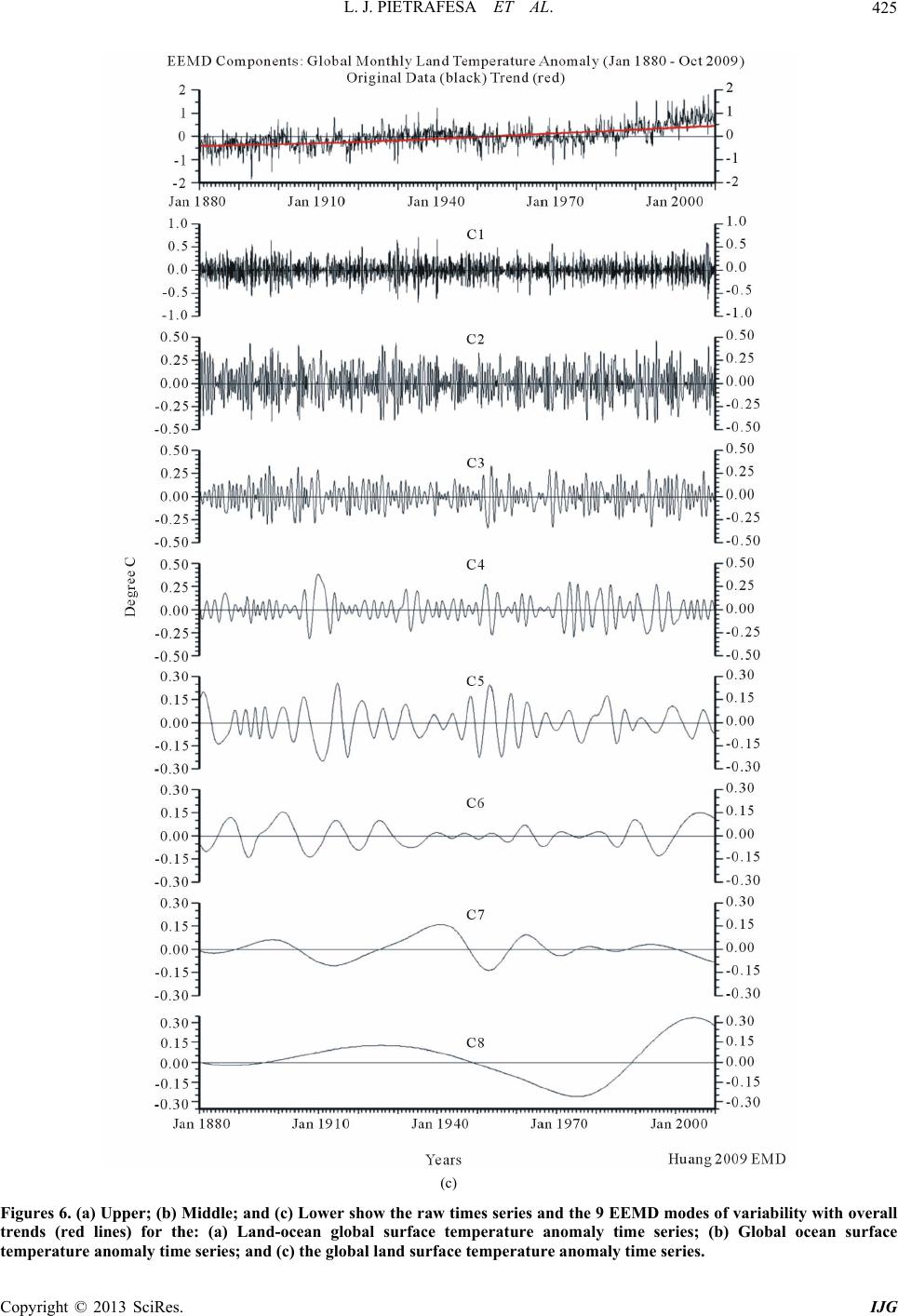 L. J. PIETRAFESA ET AL. 425 (c) Figures 6. (a) Upper; (b) Middle; and (c) Lower show the raw times series and the 9 EEMD modes of variability with overall trends (red lines) for the: (a) Land-ocean global surface temperature anomaly time series; (b) Global ocean surface emperature anomaly time series; and (c) the global land surface temperature anomaly time series. t Copyright © 2013 SciRes. IJG 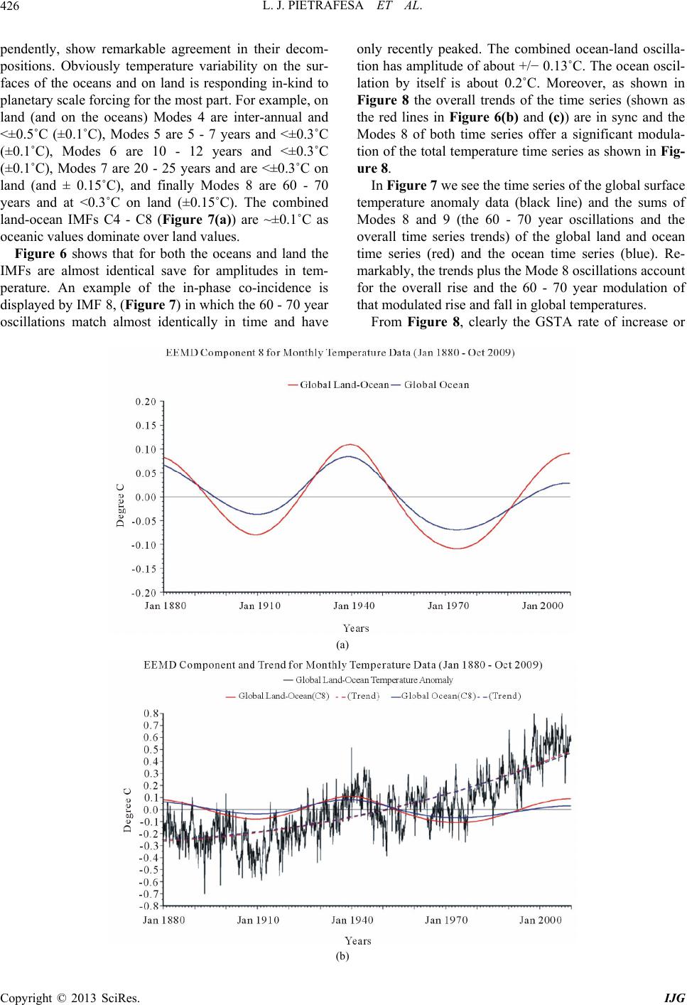 L. J. PIETRAFESA ET AL. Copyright © 2013 SciRes. IJG 426 pendently, show remarkable agreement in their decom- positions. Obviously temperature variability on the sur- faces of the oceans and on land is responding in-kind to planetary scale forcing for the most part. For example, on land (and on the oceans) Modes 4 are inter-annual and <±0.5˚C (±0.1˚C), Modes 5 are 5 - 7 years and <±0.3˚C (±0.1˚C), Modes 6 are 10 - 12 years and <±0.3˚C (±0.1˚C), Modes 7 are 20 - 25 years and are <±0.3˚C on land (and ± 0.15˚C), and finally Modes 8 are 60 - 70 years and at <0.3˚C on land (±0.15˚C). The combined land-ocean IMFs C4 - C8 (Figure 7(a)) are ~±0.1˚C as oceanic values dominate over land values. Figure 6 shows that for both the oceans and land the IMFs are almost identical save for amplitudes in tem- perature. An example of the in-phase co-incidence is displayed by IMF 8, (Figure 7) in which the 60 - 70 year oscillations match almost identically in time and have only recently peaked. The combined ocean-land oscilla- tion has amplitude of about +/− 0.13˚C. The ocean oscil- lation by itself is about 0.2˚C. Moreover, as shown in Figure 8 the overall trends of the time series (shown as the red lines in Figure 6(b) and (c)) are in sync and the Modes 8 of both time series offer a significant modula- tion of the total temperature time series as shown in Fig- ure 8. In Figure 7 we see the time series of the global surface temperature anomaly data (black line) and the sums of Modes 8 and 9 (the 60 - 70 year oscillations and the overall time series trends) of the global land and ocean time series (red) and the ocean time series (blue). Re- markably, the trends plus the Mode 8 oscillations account for the overall rise and the 60 - 70 year modulation of that modulated rise and fall in global temperatures. From Figure 8, clearly the GSTA rate of increase or (a) (b) 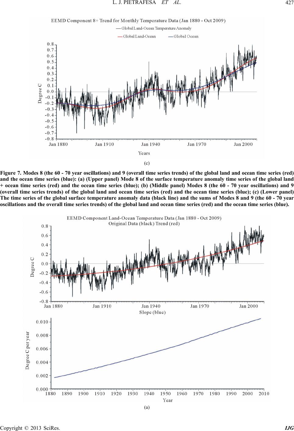 L. J. PIETRAFESA ET AL. 427 (c) Figure 7. Modes 8 (the 60 - 70 year oscillations) and 9 (overall time series trends) of the global land and ocean time series (red) and the ocean time series (blue): (a) (Upper panel) Mode 8 of the surface temperature anomaly time series of the global land + ocean time series (red) and the ocean time series (blue); (b) (Middle panel) Modes 8 (the 60 - 70 year oscillations) and 9 (overall time series trends) of the global land and ocean time series (red) and the ocean time series (blue); (c) (Lower panel) The time series of the global surface temperature anomaly data (black line) and the sums of Modes 8 and 9 (the 60 - 70 year oscillations and the overall time series trends) of the global land and ocean time series (red) and the ocean time series (blue). (a) Copyright © 2013 SciRes. IJG 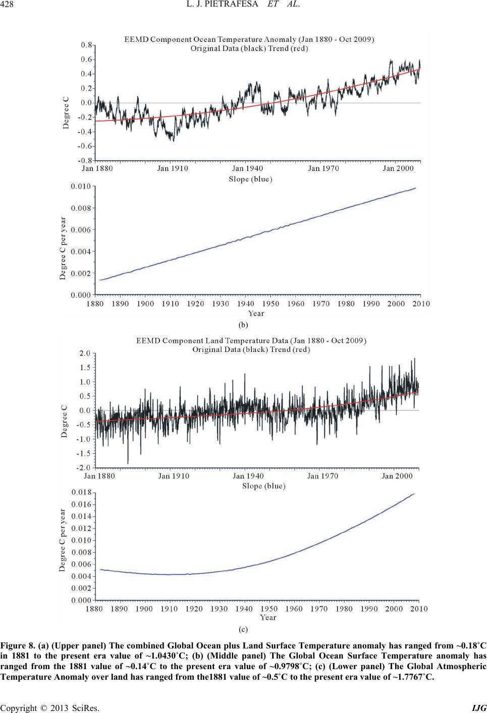 L. J. PIETRAFESA ET AL. 428 (b) (c) Figure 8. (a) (Upper panel) The combined Global Ocean plus Land Surface Temperature anomaly has ranged from ~0.18˚C in 1881 to the present era value of ~1.0430˚C; (b) (Middle panel) The Global Ocean Surface Temperature anomaly has ranged from the 1881 value of ~0.14˚C to the present era value of ~0.9798˚C; (c) (Lower panel) The Global Atmospheric emperature Anomaly over land has ranged from the1881 value of ~0.5˚C to the present era value of ~1.7767˚C. T Copyright © 2013 SciRes. IJG 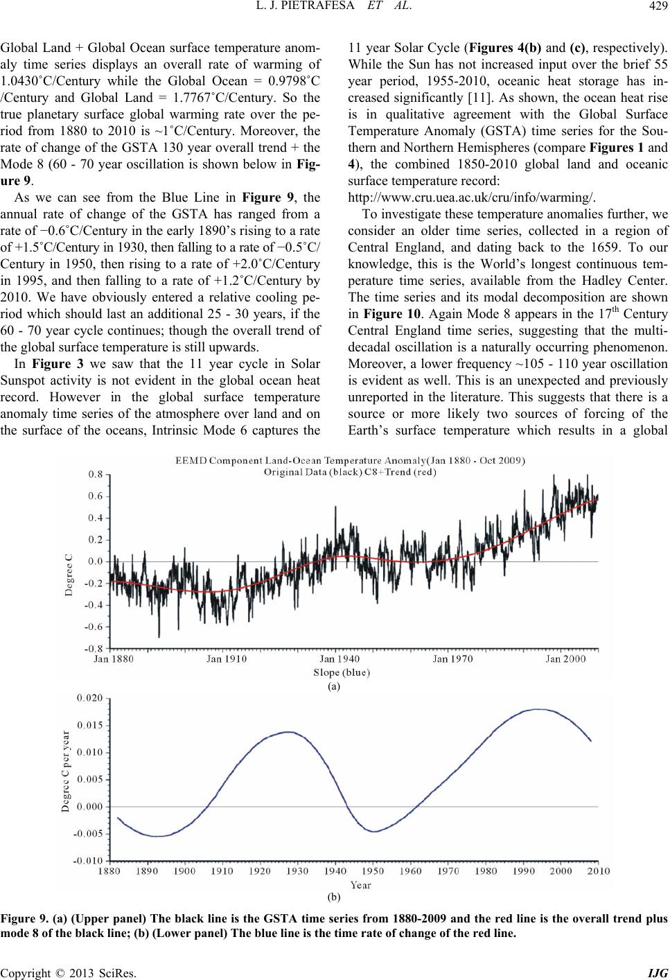 L. J. PIETRAFESA ET AL. Copyright © 2013 SciRes. IJG 429 Global Land + Global Ocean surface temperature anom- aly time series displays an overall rate of warming of 1.0430˚C/Century while the Global Ocean = 0.9798˚C /Century and Global Land = 1.7767˚C/Century. So the true planetary surface global warming rate over the pe- riod from 1880 to 2010 is ~1˚C/Century. Moreover, the rate of change of the GSTA 130 year overall trend + the Mode 8 (60 - 70 year oscillation is shown below in Fig- ure 9. As we can see from the Blue Line in Figure 9, the annual rate of change of the GSTA has ranged from a rate of −0.6˚C/Century in the early 1890’s rising to a rate of +1.5˚C/Century in 1930, then falling to a rate of −0.5˚C/ Century in 1950, then rising to a rate of +2.0˚C/Century in 1995, and then falling to a rate of +1.2˚C/Century by 2010. We have obviously entered a relative cooling pe- riod which should last an additional 25 - 30 years, if the 60 - 70 year cycle continues; though the overall trend of the global surface temperature is still upwards. In Figure 3 we saw that the 11 year cycle in Solar Sunspot activity is not evident in the global ocean heat record. However in the global surface temperature anomaly time series of the atmosphere over land and on the surface of the oceans, Intrinsic Mode 6 captures the 11 year Solar Cycle (Figures 4(b) and (c), respectively). While the Sun has not increased input over the brief 55 year period, 1955-2010, oceanic heat storage has in- creased significantly [11]. As shown, the ocean heat rise is in qualitative agreement with the Global Surface Temperature Anomaly (GSTA) time series for the Sou- thern and Northern Hemispheres (compare Figures 1 and 4), the combined 1850-2010 global land and oceanic surface temperature record: http://www.cru.uea.ac.uk/cru/info/warming/. To investigate these temperature anomalies further, we consider an older time series, collected in a region of Central England, and dating back to the 1659. To our knowledge, this is the World’s longest continuous tem- perature time series, available from the Hadley Center. The time series and its modal decomposition are shown in Figure 10. Again Mode 8 appears in the 17th Century Central England time series, suggesting that the multi- decadal oscillation is a naturally occurring phenomenon. Moreover, a lower frequency ~105 - 110 year oscillation is evident as well. This is an unexpected and previously unreported in the literature. This suggests that there is a source or more likely two sources of forcing of the Earth’s surface temperature which results in a global (a) (b) Figure 9. (a) (Upper panel) The black line is the GSTA time series from 1880-2009 and the red line is the overall trend plus mode 8 of the black line; (b) (Lower panel) The blue line is the time rate of change of the red line. 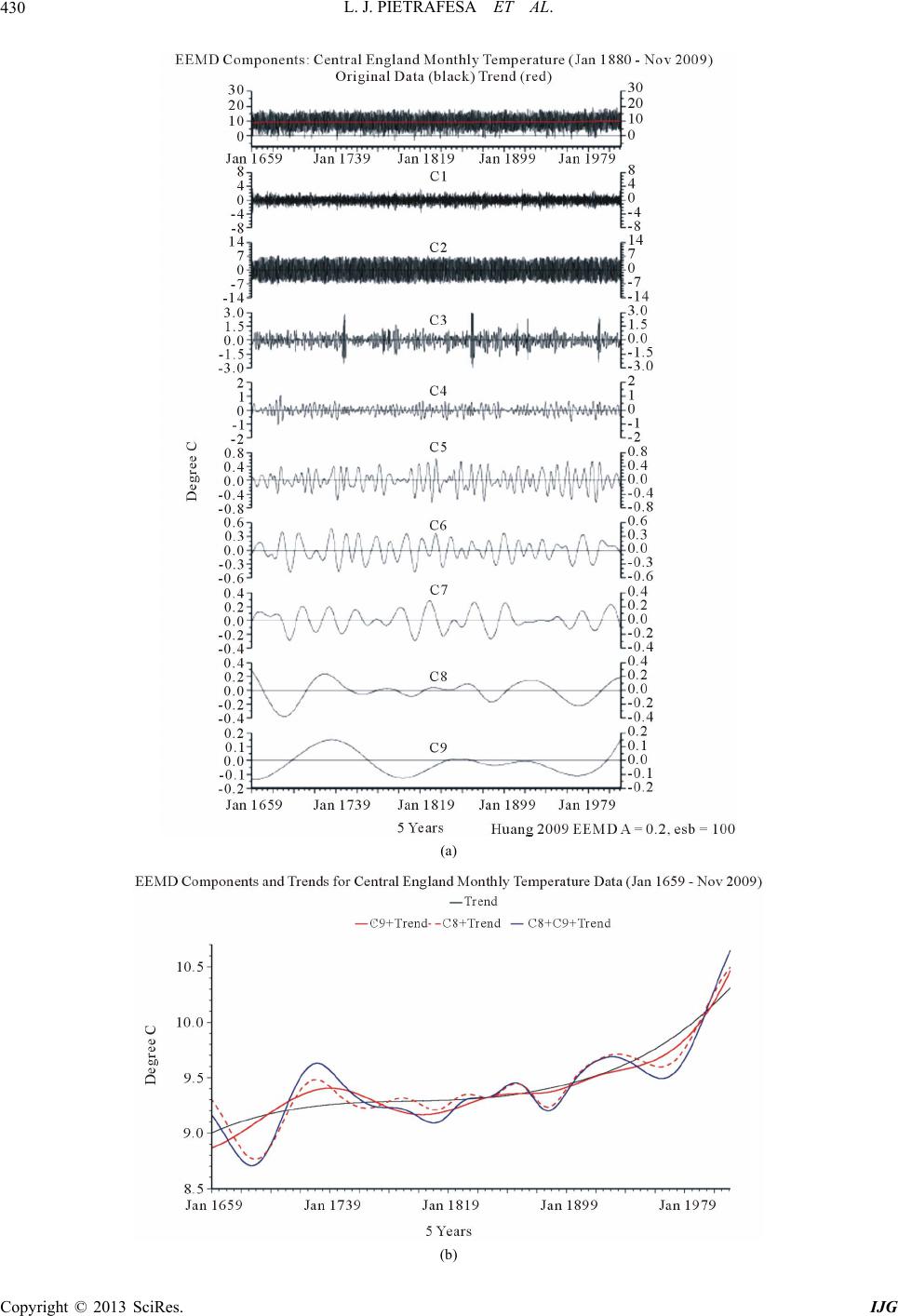 L. J. PIETRAFESA ET AL. 430 (a) (b) Copyright © 2013 SciRes. IJG 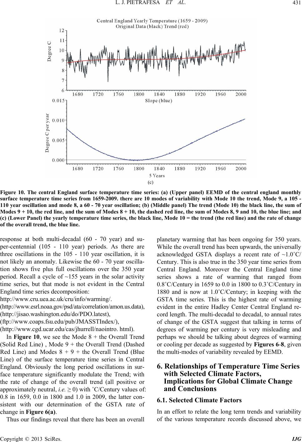 L. J. PIETRAFESA ET AL. Copyright © 2013 SciRes. IJG 431 (c) Figure 10. The central England surface temperature time series: (a) (Upper panel) EEMD of the central england monthly surface temperature time series from 1659-2009. there are 10 modes of variability with Mode 10 the trend, Mode 9, a 105 - 110 year oscillation and mode 8, a 60 - 70 year oscillation; (b) (Middle panel) The trend (Mode 10) the black line, the sum of Modes 9 + 10, the red line, and the sum of Modes 8 + 10, the dashed red line, the sum of Modes 8, 9 and 10, the blue line; and (c) (Lower Panel) the yearly temperature time series, the black line, Mode 10 = the trend (the red line) and the rate of change of the overall trend, the blue line. response at both multi-decadal (60 - 70 year) and su- per-centennial (105 - 110 year) periods. As there are three oscillations in the 105 - 110 year oscillation, it is not likely an anomaly. Likewise the 60 - 70 year oscilla- tion shows five plus full oscillations over the 350 year period. Recall a cycle of ~155 years in the solar activity time series, but that mode is not evident in the Central England time series decomposition: http://www.cru.uea.ac.uk/cru/info/warming/. (http://www.esrl.noaa.gov/psd/ata/correlation/amon.us.data), (http://jisao.wash ington.edu/do/PDO.latest), (ftp://www.coaps.fsu.edu/pub/JMASSTIndex/), (http://www.cgd.ucar.edu/cas/jhurrell/naointro. html). In Figure 10, we see the Mode 8 + the Overall Trend (Solid Red Line) , Mode 9 + the Overall Trend (Dashed Red Line) and Modes 8 + 9 + the Overall Trend (Blue Line) of the surface temperature time series in Central England. Obviously the long period oscillations in sur- face temperature significantly modulate the Trend; with the rate of change of the overall trend (all positive or approximately neutral, i.e. ≥ 0) with ˚C/Century values of: 0.8 in 1659, 0.0 in 1800 and 1.0 in 2009, the latter con- sistent with our determination of the GSTA rate of change in Figure 6(a). Thus our findings reveal that there has been an overall planetary warming that has been ongoing for 350 years. While the overall trend has been upwards, the universally acknowledged GSTA displays a recent rate of ~1.0˚C/ Century. This is also true in the 350 year time series from Central England. Moreover the Central England time series shows a rate of warming that ranged from 0.8˚C/Century in 1659 to 0.0 in 1800 to 0.3˚C/Century in 1880 and is now at 1.0˚C/Century; in keeping with the GSTA time series. This is the highest rate of warming evident in the entire Hadley Center Central England re- cord length. The multi-decadal to decadal, to annual rates of change of the GSTA suggest that talking in terms of degrees of warming per century is very misleading and perhaps we should be talking about degrees of warming or cooling per decade as suggested by Figures 6-8, given the multi-modes of variability revealed by EEMD. 6. Relationships of Temperature Time Series with Selected Climate Factors, Implications for Global Climate Change and Conclusions 6.1. Selected Climate Factors In an effort to relate the long term trends and variability of the various temperature records discussed above, we  L. J. PIETRAFESA ET AL. 432 next consider their possible correlations with climate factor behavior over the record lengths of the data from which they are derived. We will consider the North At- lantic Oscillation (NAO), the Pacific Decadal Oscillation (PDO), the Atlantic Multi-Decadal Oscillation (AMO), the El Niño Southern Oscillation/Japan Meteorological Agency (ENSO/JMA), the Arctic Oscillation (AO), the Quasi-Biennial Oscillation, Sun Spot Activity, and the Atlantic Meridional Mode (AMM). We present the time series and modal decompositions of these factors in Fig- ure 9. The NAO is traditionally defined as the normalized pressure difference between a station on the Azores and one at Reykjavik, Iceland. The NAO is the dominant mode of winter climate variability in the North Atlantic region ranging from central North America to Europe and much into Northern Asia, which is defined by the pressure difference between the Azores and Iceland. An extended version of the index can be derived for the winter half of the year by using a station in the south- western part of the Iberian Peninsula [12]. Here we give data for SW Iceland (Reykjavik), Gibraltar and Ponta Delgada (Azores) as calculated by [13]. The AO is an atmospheric circulation pattern in which the atmospheric pressure over the polar regions varies in opposition with that over middle latitudes (about 45 de- grees North) on time scales ranging from weeks to dec- ades. The AO is the projection of monthly mean 1000 mb height anomalies onto the 1st EOF poleward of 20-de- grees North. Values are normalized by the 1979-2000 period. The AO is the dominant pattern of non-seasonal Sea-Level Pressure (SLP) variations north of 20N, and it is characterized by SLP anomalies of one sign in the Arctic and anomalies of opposite sign centered about 37 - 45N. The AO oscillation extends through the depth of the troposphere. During the months of January through March it extends upward into the stratosphere where it modulates in the strength of the westerly vortex that en- circles the Arctic polar cap region. The NAO and the AO are different ways of describing the same phenomenon. The Pacific Decadal Oscillation (PDO) Index is de- fined as the leading principal component of North Pacific monthly sea surface temperature variability (poleward of 20N for the 1900-93 period) [14]: While ENSO and the PDO have similar spatial climate fingerprints, they have very different behavior in time. The indices of PDO and ENSO are significantly correlated. The Atlantic Multi-decadal Oscillation (AMO) repre- sents a cycle in the large-scale atmospheric flow and ocean currents in the North Atlantic Ocean that combine to alternately increase and decrease Atlantic sea surface temperatures (SSTs). It is defined as the mean SST be- tween 75˚W and 7.5˚W and south of 60˚N, and has been identified to have a close relationship with Sahara rain- fall and Atlantic dipole mode. The AMO is the time se- ries calculated from the Kaplan SST dataset and is up- dated monthly www.esrl.noaa.gov/psd/data/gridded/data.kalan_sst.html. For ENSO, we employ the Japan Meteorological Agency (JMA) Index which is based on an SST-based index for determining El Nino and La Nina-El Viejo events [15] JMA calculates monthly SST anomalies av- eraged for the area 4 N to 4 S and 150 W to 90 W. Also applied is a 5-month running mean of the data. The 5-month running mean is implemented to smooth out possible intra-seasonal variations. The AMO un-smoothed version is at: http://www.esrl.noaa.gov/psd/data/correlation/amon.us.data. The PDO Index data can be found on the web: http://jisao.washington.edu/pdo/PDO latest. As stated in the website, “the updated standardized values for the PDO Index, derived as the leading Principle Component of monthly SST anomalies in the North Pacific Ocean, pole ward of 20N. The monthly mean global average SST anomalies are removed to separate this pattern of variability from any “global warming” signal that may be present in the data. We were not able to find an un-smoothed version of the PDO. The JMA ENSO index can be found at: ftp://www.coaps.fsu.edu/pub/JMA_ SST_Index/ The jmasst1868-today.filter-5 is the only unsmoothed time series. As we can see from the RE- ADME file: The data file (jmasst1868-today.filter-5) is the JMA index based on reconstructed monthly mean SST fields for the period Jan. 1868 - Feb. 1949 and on the ob- served JMA SST index for March 1949 to the present. The Quasi-Biennial Oscillation (QBO) is defined as a quasi-periodic oscillation of the equatorial zonal wind between easterlies and westerlies in the tropical strato- sphere with a mean period of 28 to 29 months. The al- ternating wind regimes develop at the top of the lower stratosphere and propagate downwards at about 1 km (0.6 mi) per month until they are dissipated at the tropical tropopause. Downward motion of the easterlies is usually more irregular than that of the westerlies. The amplitude of the easterly phase is about twice as strong as that of the westerly phase. At the top of the vertical QBO do- main, easterlies dominate, while at the bottom, westerlies are more likely to be found. The data are available from NCAR at: climatedataguide.ucar.edu/guidance/qbo-quasi- biennial-oscillation The following statement is from NCAR: http://www. cgd.ucar.edu/cas/jhurrell/naointro.html “Since there is no unique way to define the spatial structure of the NAO, it follows that there is no univer- sally accepted index to describe the temporal evolution of the phenomenon. Most modern NAO indices are de- rived either from the simple difference in surface pres- sure anomalies between various northern and southern Copyright © 2013 SciRes. IJG 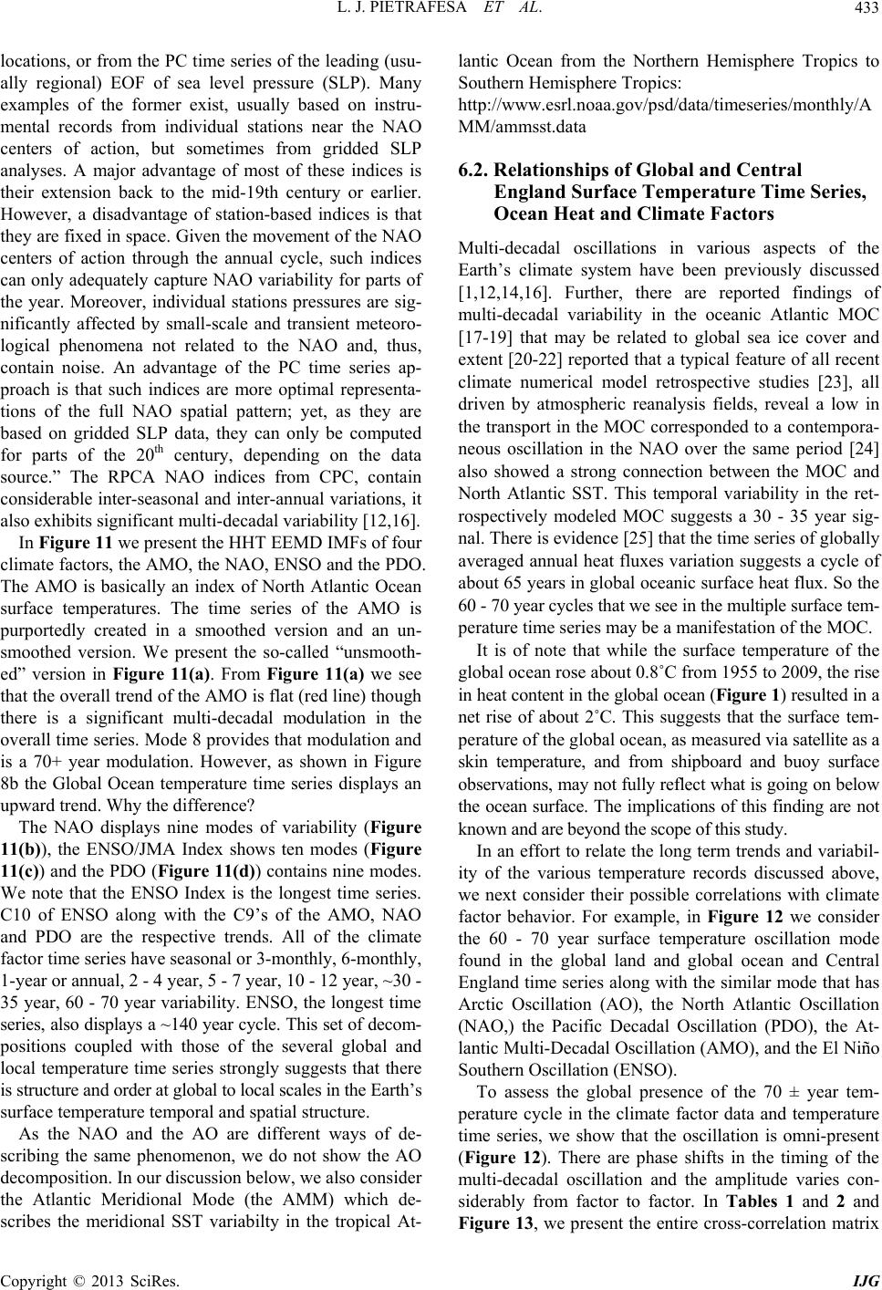 L. J. PIETRAFESA ET AL. 433 locations, or from the PC time series of the leading (usu- ally regional) EOF of sea level pressure (SLP). Many examples of the former exist, usually based on instru- mental records from individual stations near the NAO centers of action, but sometimes from gridded SLP analyses. A major advantage of most of these indices is their extension back to the mid-19th century or earlier. However, a disadvantage of station-based indices is that they are fixed in space. Given the movement of the NAO centers of action through the annual cycle, such indices can only adequately capture NAO variability for parts of the year. Moreover, individual stations pressures are sig- nificantly affected by small-scale and transient meteoro- logical phenomena not related to the NAO and, thus, contain noise. An advantage of the PC time series ap- proach is that such indices are more optimal representa- tions of the full NAO spatial pattern; yet, as they are based on gridded SLP data, they can only be computed for parts of the 20th century, depending on the data source.” The RPCA NAO indices from CPC, contain considerable inter-seasonal and inter-annual variations, it also exhibits significant multi-decadal variability [12,16]. In Figure 11 we present the HHT EEMD IMFs of four climate factors, the AMO, the NAO, ENSO and the PDO. The AMO is basically an index of North Atlantic Ocean surface temperatures. The time series of the AMO is purportedly created in a smoothed version and an un- smoothed version. We present the so-called “unsmooth- ed” version in Figure 11(a). From Figure 11(a) we see that the overall trend of the AMO is flat (red line) though there is a significant multi-decadal modulation in the overall time series. Mode 8 provides that modulation and is a 70+ year modulation. However, as shown in Figure 8b the Global Ocean temperature time series displays an upward trend. Why the difference? The NAO displays nine modes of variability (Figure 11(b)), the ENSO/JMA Index shows ten modes (Figure 11(c)) and the PDO (Figure 11(d)) contains nine modes. We note that the ENSO Index is the longest time series. C10 of ENSO along with the C9’s of the AMO, NAO and PDO are the respective trends. All of the climate factor time series have seasonal or 3-monthly, 6-monthly, 1-year or annual, 2 - 4 year, 5 - 7 year, 10 - 12 year, ~30 - 35 year, 60 - 70 year variability. ENSO, the longest time series, also displays a ~140 year cycle. This set of decom- positions coupled with those of the several global and local temperature time series strongly suggests that there is structure and order at global to local scales in the Earth’s surface temperature temporal and spatial structure. As the NAO and the AO are different ways of de- scribing the same phenomenon, we do not show the AO decomposition. In our discussion below, we also consider the Atlantic Meridional Mode (the AMM) which de- scribes the meridional SST variabilty in the tropical At- lantic Ocean from the Northern Hemisphere Tropics to Southern Hemisphere Tropics: http://www.esrl.noaa.gov /psd/data/timeseries/month ly/A MM/ammsst.data 6.2. Relationships of Global and Central England Surface Temperature Time Series, Ocean Heat and Climate Factors Multi-decadal oscillations in various aspects of the Earth’s climate system have been previously discussed [1,12,14,16]. Further, there are reported findings of multi-decadal variability in the oceanic Atlantic MOC [17-19] that may be related to global sea ice cover and extent [20-22] reported that a typical feature of all recent climate numerical model retrospective studies [23], all driven by atmospheric reanalysis fields, reveal a low in the transport in the MOC corresponded to a contempora- neous oscillation in the NAO over the same period [24] also showed a strong connection between the MOC and North Atlantic SST. This temporal variability in the ret- rospectively modeled MOC suggests a 30 - 35 year sig- nal. There is evidence [25] that the time series of globally averaged annual heat fluxes variation suggests a cycle of about 65 years in global oceanic surface heat flux. So the 60 - 70 year cycles that we see in the multiple surface tem- perature time series may be a manifestation of the MOC. It is of note that while the surface temperature of the global ocean rose about 0.8˚C from 1955 to 2009, the rise in heat content in the global ocean (Figure 1) resulted in a net rise of about 2˚C. This suggests that the surface tem- perature of the global ocean, as measured via satellite as a skin temperature, and from shipboard and buoy surface observations, may not fully reflect what is going on below the ocean surface. The implications of this finding are not known and are beyond the scope of this study. In an effort to relate the long term trends and variabil- ity of the various temperature records discussed above, we next consider their possible correlations with climate factor behavior. For example, in Figure 12 we consider the 60 - 70 year surface temperature oscillation mode found in the global land and global ocean and Central England time series along with the similar mode that has Arctic Oscillation (AO), the North Atlantic Oscillation (NAO,) the Pacific Decadal Oscillation (PDO), the At- lantic Multi-Decadal Oscillation (AMO), and the El Niño Southern Oscillation (ENSO). To assess the global presence of the 70 ± year tem- perature cycle in the climate factor data and temperature time series, we show that the oscillation is omni-present (Figure 12). There are phase shifts in the timing of the multi-decadal oscillation and the amplitude varies con- siderably from factor to factor. In Tables 1 and 2 and Figure 13, we present the entire cross-correlation matrix Copyright © 2013 SciRes. IJG 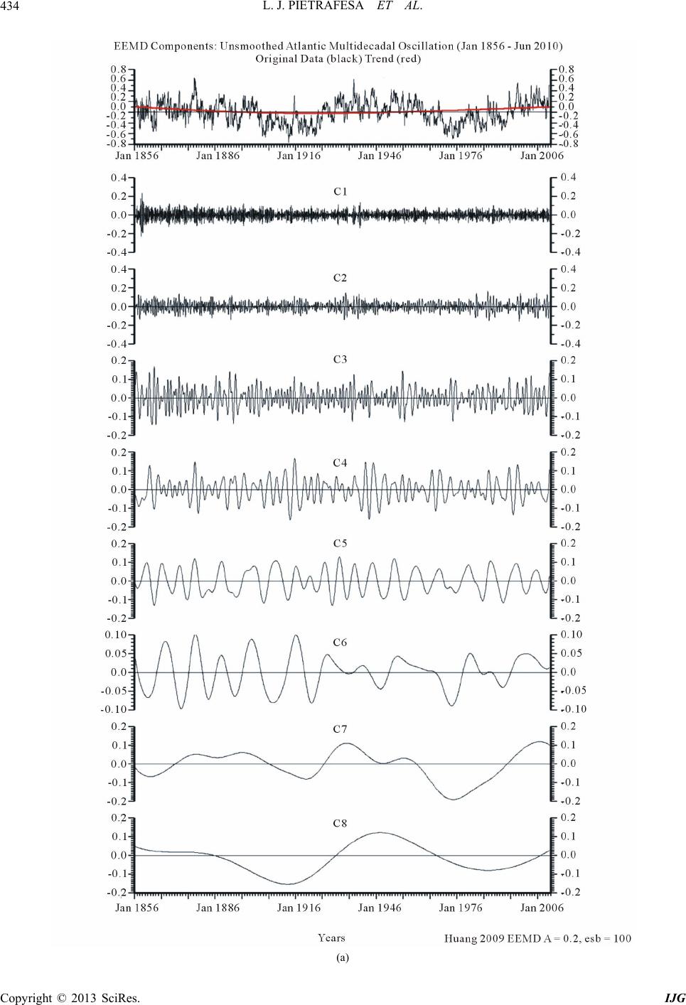 L. J. PIETRAFESA ET AL. Copyright © 2013 SciRes. IJG 434 (a) 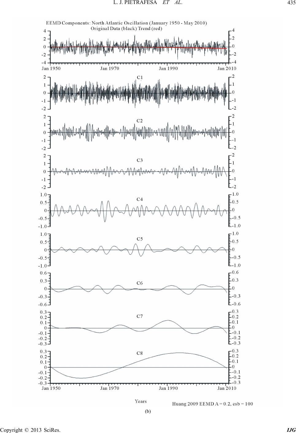 L. J. PIETRAFESA ET AL. 435 (b) Copyright © 2013 SciRes. IJG 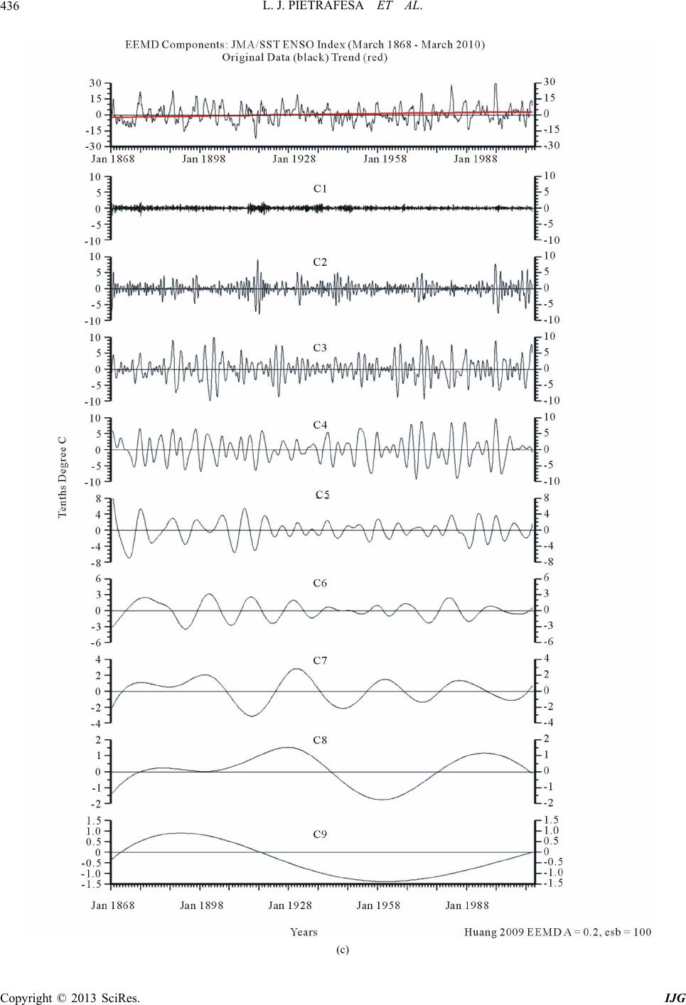 L. J. PIETRAFESA ET AL. 436 (c) Copyright © 2013 SciRes. IJG 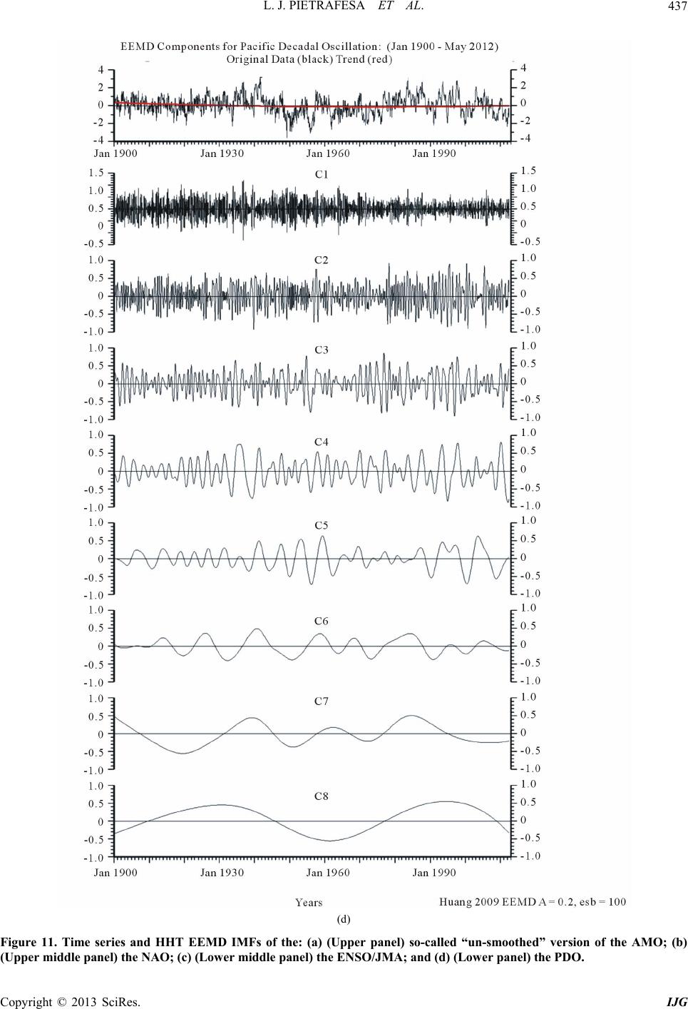 L. J. PIETRAFESA ET AL. 437 (d) Figure 11. Time series and HHT EEMD IMFs of the: (a) (Upper panel) so-called “un-smoothed” version of the AMO; (b) (Upper middle panel) the NAO; (c) (Lower middle panel) the ENSO/JMA; and (d) (Lower panel) the PDO. Copyright © 2013 SciRes. IJG 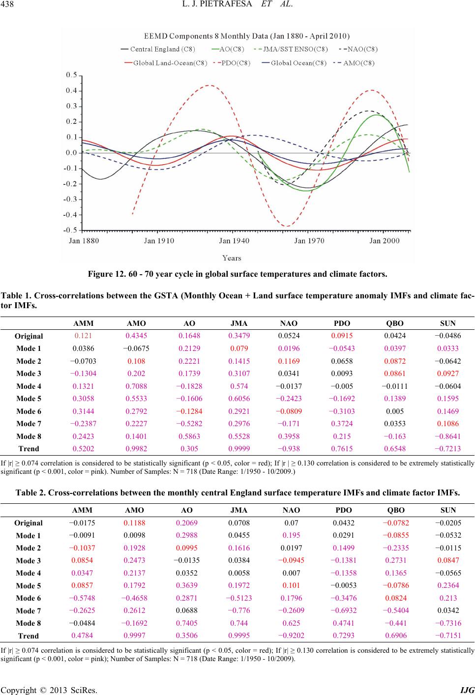 L. J. PIETRAFESA ET AL. 438 Figure 12. 60 - 70 year cycle in global surface temperatures and climate factors. Table 1. Cross-correlations between the GSTA (Monthly Ocean + Land surface temperature anomaly IMFs and climate fac- tor IMFs. AMM AMO AO JMA NAO PDO QBO SUN Original 0.121 0.4345 0.1648 0.3479 0.0524 0.0915 0.0424 −0.0486 Mode 1 0.0386 −0.0675 0.2129 0.079 0.0196 −0.0543 0.0397 0.0333 Mode 2 −0.0703 0.108 0.2221 0.1415 0.1169 0.0658 0.0872 −0.0642 Mode 3 −0.1304 0.202 0.1739 0.3107 0.0341 0.0093 0.0861 0.0927 Mode 4 0.1321 0.7088 −0.1828 0.574 −0.0137 −0.005 −0.0111 −0.0604 Mode 5 0.3058 0.5533 −0.1606 0.6056 −0.2423 −0.1692 0.1389 0.1595 Mode 6 0.3144 0.2792 −0.1284 0.2921 −0.0809 −0.3103 0.005 0.1469 Mode 7 −0.2387 0.2227 −0.5282 0.2976 −0.171 0.3724 0.0353 0.1086 Mode 8 0.2423 0.1401 0.5863 0.5528 0.3958 0.215 −0.163 −0.8641 Trend 0.5202 0.9982 0.305 0.9999 −0.938 0.7615 0.6548 −0.7213 If |r| ≥ 0.074 correlation is considered to be statistically significant (p < 0.05, color = red); If |r | ≥ 0.130 correlation is considered to be extremely statistically significant (p < 0.001, color = pink). Number of Samples: N = 718 (Date Range: 1/1950 - 10/2009.) Table 2. Cross-correlations between the monthly central England surface temperature IMFs and climate factor IMFs. AMM AMO AO JMA NAO PDO QBO SUN Original −0.0175 0.1188 0.2069 0.0708 0.07 0.0432 −0.0782 −0.0205 Mode 1 −0.0091 0.0098 0.2988 0.0455 0.195 0.0291 −0.0855 −0.0532 Mode 2 −0.1037 0.1928 0.0995 0.1616 0.0197 0.1499 −0.2335 −0.0115 Mode 3 0.0854 0.2473 −0.0135 0.0384 −0.0945 −0.1381 0.2731 0.0847 Mode 4 0.0347 0.2137 0.0352 0.0058 0.007 −0.1358 0.1365 −0.0565 Mode 5 0.0857 0.1792 0.3639 0.1972 0.101 −0.0053 −0.0786 0.2364 Mode 6 −0.5748 −0.4658 0.2871 −0.5123 0.1796 −0.3476 0.0824 0.213 Mode 7 −0.2625 0.2612 0.0688 −0.776 −0.2609 −0.6932 −0.5404 0.0342 Mode 8 −0.0484 −0.1692 0.7405 0.744 0.625 0.4741 −0.441 −0.7316 Trend 0.4784 0.9997 0.3506 0.9995 −0.9202 0.7293 0.6906 −0.7151 If |r| ≥ 0.074 correlation is considered to be statistically significant (p < 0.05, color = red); If |r| ≥ 0.130 correlation is considered to be extremely statistically significant (p < 0.001, color = pink); Number of Samples: N = 718 (Date Range: 1/1950 - 10/2009). Copyright © 2013 SciRes. IJG 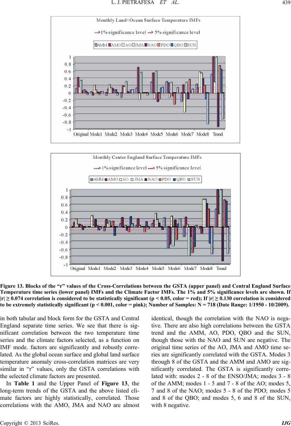 L. J. PIETRAFESA ET AL. Copyright © 2013 SciRes. IJG 439 Figure 13. Blocks of the “r” values of the Cross-Correlations between the GSTA (upper panel) and Central England Surface Temperature time series (lower panel) IMFs and the Climate Factor IMFs. The 1% and 5% significance levels are shown. If |r| ≥ 0.074 correlation is considered to be statistically significant (p < 0.05, color = red); If |r| ≥ 0.130 correlation is considered to be extremely statistically significant (p < 0.001, color = pink); Number of Samples: N = 718 (Date Range: 1/1950 - 10/2009). in both tabular and block form for the GSTA and Central England separate time series. We see that there is sig- nificant correlation between the two temperature time series and the climate factors selected, as a function on IMF mode. factors are significantly and robustly corre- lated. As the global ocean surface and global land surface temperature anomaly cross-correlation matrices are very similar in “r” values, only the GSTA correlations with the selected climate factors are presented. In Table 1 and the Upper Panel of Figure 13, the long-term trends of the GSTA and the above listed cli- mate factors are highly statistically, correlated. Those correlations with the AMO, JMA and NAO are almost identical, though the correlation with the NAO is nega- tive. There are also high correlations between the GSTA trend and the AMM, AO, PDO, QBO and the SUN, though those with the NAO and SUN are negative. The original time series of the AO, JMA and AMO time se- ries are significantly correlated with the GSTA. Modes 3 through 8 of the GSTA and the AMM and AMO are sig- nificantly correlated. The GSTA is significantly corre- lated with: modes 2 - 8 of the ENSO/JMA; modes 3 - 8 of the AMM; modes 1 - 5 and 7 - 8 of the AO; modes 5, 7 and 8 of the NAO; modes 5 - 8 of the PDO; modes 5 and 8 of the QBO; and modes 5, 6 and 8 of the SUN, with 8 negative.  L. J. PIETRAFESA ET AL. 440 In Ta ble 2 and the Lower Panel of Figure 13, and identical to that of the GSTA, the long-term trends of the GSTA and the above listed climate factors are highly statistically, correlated. Those correlations with the AMO, JMA and NAO are almost identical, though the correla- tion with the NAO is negative. There are also high cor- relations between the Central England trend and the AMM, AO, PDO, QBO and the SUN, though those with the NAO and SUN are negative. The original time series of the Central England time series is only significantly correlated with the AO. The Central England IMF modes are significantly correlated with: is significantly corre- lated with: modes 5 and 6 of the AMM; modes 2 - 8 of the AMO, with modes 6 and 8 negatively correlated; modes 2 and 5 - 8, of the ENSO/JMA modes, with 6 and 7 being negative; modes 1, 5, 6 and 8 of the AO; modes 1 and 6 - 8 of the NAO, with 7 negative; modes 2 - 4 and 6 - 8 of the PDO, with 3, 4, 6 and 7 negative; modes 2, 3, 4 and 7, 8 of the QBO, with 2, 7 and 8 negative; and modes 5, 6 and 8 of the SUN, with 8 negative. So, in general, the HHT/EEMD/IMFs of the GSTA and the Central England times series are highly corre- lated with multiple modes of the selected climate factor IMFs. Curiously modes 5 and 8 of both temperature time series are highly correlated with those of all of the cli- mate factor modes in kind. Recall that mode 5 has a 5 - 7 year cycle and mode 8 is a 60 - 70 year cycle. Mode 5 tends to be identified with ENSO while mode 8 is identi- fied with the MOC. As we discussed previously, such phenomena as West- ern Boundary Currents and the MOC, contribute to the Earth’s climate system as capacitors and as global tem- perature thermostats. The global ocean participates in the planetary climate system in several ways: exchange of heat, water vapor and CO2 with the cryosphere and at- mosphere; storage and sequestering of heat, saltwater and freshwater and CO2 and carbon at varying depths over differing time periods; and redistribution of heat, saltwa- ter, freshwater, CO2 and carbon in other forms via large scale ocean current systems. Heat and energy are redis- tributed, from the equatorial zone to the Polar zones via atmospheric eddies, aka “atmospheric storms”, which form when the ocean releases heat and moisture into the atmosphere. As relates to the MOC, climate model output is pre- sented [26] which shows a prominent quasi-decadal os- cillation in modeled SSTs, in keeping with IMF Mode 8. However, and unfortunately, the scientific literature con- tains only a crude, rudimentary picture of the MOC and other global ocean thermohaline circulations (the THC) and thus redistributions of heat, salt and buoyancy based on observations. So the true pictures of processes and time-scales of ocean phenomena, even those coupled to the atmosphere, remains unresolved. However, it is also clear that this multi-decadal cycle is vitally important to the disposition of global surface temperatures and as such, any future freshening of the North Atlantic Ocean via glacial melting could slow the strength and speed of the MOC down and thus affect our future climate. This speaks to the need of more and better observations, in- formation and numerical modeling of the MOC. Albeit, there are concerns being expressed about the uncertainty surrounding the future of the MOC [27]. 6.3. Implications for Global Climate Change It has been suggested [19] that strong multi-decadal and centennial time scale variability could mask anthropo- genic climate signals which have evolved over similar time scales. We have shown (Figure 7) that this has hap- pened with the positive cycle of Mode 8 having occurred in the late 20th Century and several years into the 21st Century, thus having suggested a higher rate of rise of GSTA then should have been computed via a properly computed trend. However, by conducting the HHT EEMD IMF modal decompositions shown in Figures 8 and 10 we have essentially removed all NS modes or variability from the total GSTA and Central England Temperature time series. The GSTA and Central England trend curves are still NL. In Figure 14 the curves of the overall trends of the GSTA and the Central England Temperature time series with the Carbon Loading Curve. The GSTA and CO2 curve, Figure 14(a), are well aligned and seemingly overlay from 1880 to the 1910s and then again in the early 1970s to the mid-2000s; in each case before and after which there is curve to curve divergence. Likewise the Central England time series trend follows the in- crease in CO2 but locks into the CO2 curve from the 1970s onward. In Figure 14, we demonstrate that by employing HHT/ EEMD, we have produced the trends of the GSTA and Central England temperature time series. GSTA and Central England surface temperature trends and the car- bon loading time series, represented as increases in CO2 are highly correlated. If we now consider the integral of the carbon loading curve scaled from 1880 to 2007 (the last year for which carbon data are available), with the time interval of one year, the integral of the carbon load- ing curve from 1880 to 2007 is the sum of those years’ loading, which is 332,472 million (106) Metric Tons of Carbon (MMTCs). The recent rate of loading of about 8.5 MMTC/Year so the total Carbon Loading from 1880-2009 is 332.489 Billion Metric Tons of Carbon (BMTCs). If we then relate this number to the overall trend in the GSTA time series, which is a commensurate rise, we can compute a relationship between the two curves, from 1880-2009, of 2.152676 (10−3)˚C/BMTC of Fossil Fuels burned. (The equ valent Fahrenheit units are i Copyright © 2013 SciRes. IJG 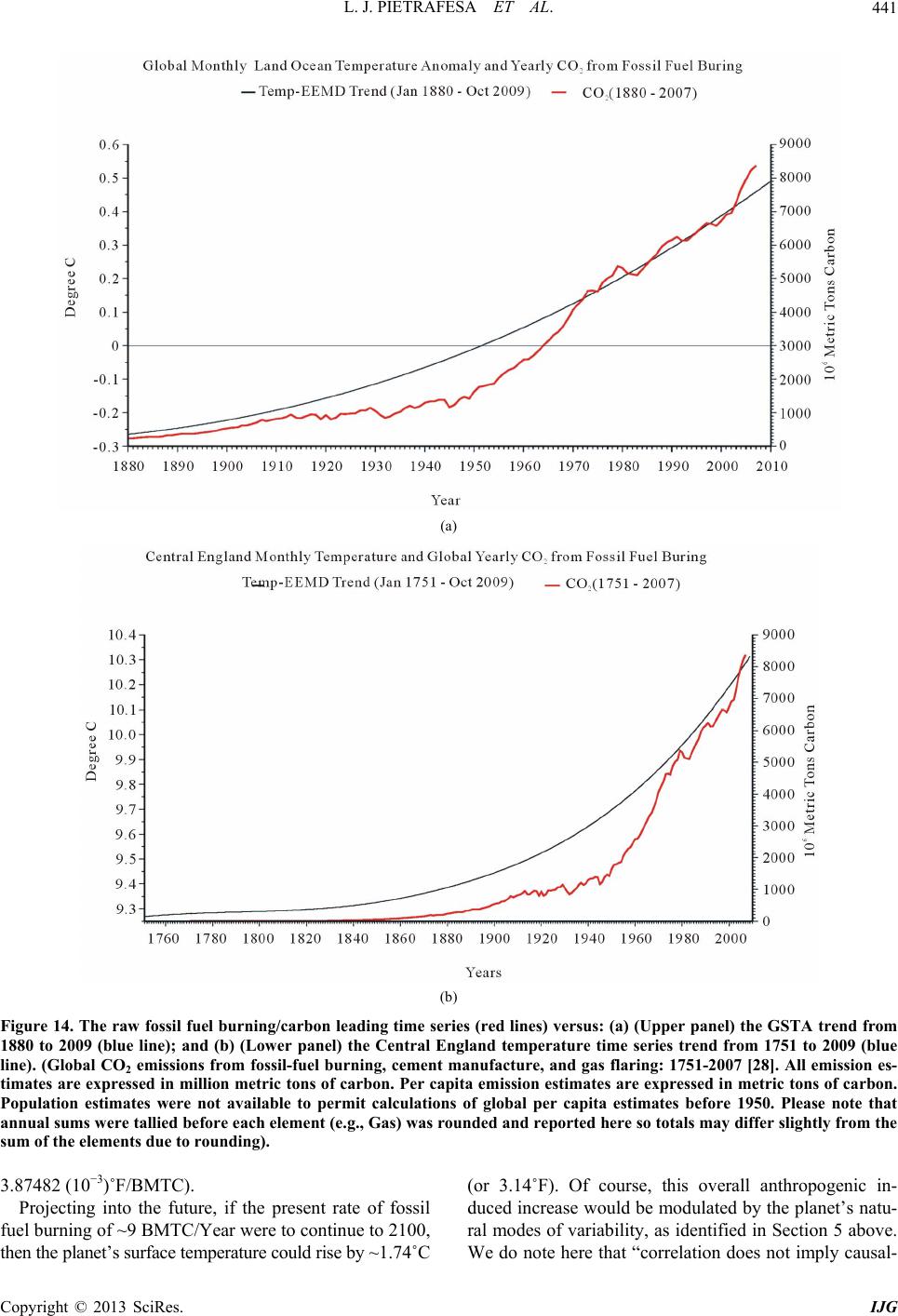 L. J. PIETRAFESA ET AL. Copyright © 2013 SciRes. IJG 441 (a) (b) Figure 14. The raw fossil fuel burning/carbon leading time series (red lines) versus: (a) (Upper panel) the GSTA trend from 1880 to 2009 (blue line); and (b) (Lower panel) the Central England temperature time series trend from 1751 to 2009 (blue line). (Global CO2 emissions from fossil-fuel burning, cement manufacture, and gas flaring: 1751-2007 [28]. All emission es- timates are expressed in million metric tons of carbon. Per capita emission estimates are expressed in metric tons of carbon. Population estimates were not available to permit calculations of global per capita estimates before 1950. Please note that annual sums were tallied before each element (e.g., Gas) was rounded and reported here so totals may differ slightly from the sum of the elements due to rounding). 3.87482 (10−3)˚F/BMTC). Projecting into the future, if the present rate of fossil fuel burning of ~9 BMTC/Year were to continue to 2100, then the planet’s surface temperature could rise by ~1.74˚C (or 3.14˚F). Of course, this overall anthropogenic in- duced increase would be modulated by the planet’s natu- ral modes of variability, as identified in Section 5 above. We do note here that “correlation does not imply causal-  L. J. PIETRAFESA ET AL. 442 ity” [29] and that a system as complex of the Earth’s Climate system can make adjustments to continued or increased fossil fuel burning, in ways that we can only speculate upon at present; even given our growing ena- bling capability to numerically model the future tem- perature of our planet. 6.4. Conclusions In the time series of global ocean and land/atmospheric and Central England surface temperatures, there are higher to lower frequency modes of variability that are superimposed on each other. The lowest frequency mode is the overall trend of the time series. There is no a priori reason for energy to be constrained to move either up or down the energy spectrum and can exist at definitive frequencies and presumably be transferred up or down the energy spectrum. The global ocean is the leading heat sink and source for the planet’s climate variability. Land surface tem- peratures have increased at the rate of 1.78˚C/Century. Ocean surface temperatures have increased at the rate of 0.98˚C/Century. The planetary surface has been warming at an overall rate of 1.04˚C/Century, more in keeping with the global ocean increase than the surface tempera- tures on land. So the global Ocean is modulating or con- trolling the planetary surface temperature; to wit the Ocean may be controlling the planetary surface tempera- tures. Our study shows that there are seasonal, twice yearly, annual, inter-annual, 5 - 7 year, 10 - 12 year, 30 - 35 year and 60 - 70 year oscillations in the planetary surface tem- perature record. The 60 - 70 year signal strongly modu- lates the running trend of the overall warming of the planet. Unfortunately this 60 - 70 year global surface temperature oscillation cannot be causally identified and proven with existing oceanic data sets as observations in the global oceans are sorely lacking. However, shorter time series of global and regional temperature and salin- ity data sets and global surface heat flux data sets are encouraging that this feature does exist in relationship to the Atlantic MOC. This oceanic feature has also ap- peared in numerical model output [19-22] and may be tied to a fundamental time scale of the MOC. These modeling studies make the case for the need for truly inter-actively coupled atmospheric-oceanic models and more aggressive global ocean observational programs, needed to reveal more about our climate system; given the paucity of oceanic data. Known climate factors consist of multiple modes of variability. Carbon loading appears to have a strong sig- nal in the Earth’s surface temperature record. As we have burned nearly 350 billion metric tons of fossil fuels over the Industrial Age, that release of Carbon appears to have resulted in a direct net increase of about 0.7523˚C of the Earth’s surface temperature; much of the globally ob- served surface temperature increase. Presently the rate of fossil fuel burning is ~9 BMTC/Year and could lead to a human caused increase in the Earth’s surface temperature of ~1.74˚C by the onset of the 22nd Century, if recent past is prologue to the future. 7. Acknowledgements The US DoD agency DARPA provided the support for this study. Dr. N.E. Huang and Dr. Z. Wu are acknowl- edged for insightful discussions regarding the Earth’s climate system. We would also like to acknowledge those committed individuals who gave their time and effort to making those surface temperature measurements for over three and a half millennia. REFERENCES [1] K. E. Trenberth, D. P. Stepaniak and J. M. Caron, “Inter- annual Variations in the Atmospheric Heat Budget,” Journal of Geophysical Research, Vol. 107, No. D8, 2002, pp. AAC 4-1-AAC 4-15. doi:10.1029/2000JD000297 [2] K. E. Trenberth, “Handbook of Weather,” In: T. D. Potter and B. R. Coleman, Eds., Climate and Water, John Wiley and Sons, Hoboken, 2003, pp. 163-173. [3] J. M. Vogel and B. Lazar, “Global Cooling, Science and Myth,” Weatherwise, Vol. 63, No. 4, 2010, pp. 24-31. doi:10.1080/00431672.2010.490166 [4] S. Levitus, J. Antonov and T. Boyer, “Warming of the world ocean, 1955-2003,” Geophysical Research Letters, Vol. 32, No. 2, 2005, Article ID: L02604. doi:10.1029/2004GL021592 [5] N. E. Huang, Z. Shen, S. R. Long, M. L. Wu, H. H. Shih, Q. Zheng, N. C. Yen, C. C. Tung and H. H. Liu, “The Empirical Mode Decompostion and Hilbert Spectrum for Nonlinear and Nonstationary Time Series Analysis,” Proceedings of the Royal Society A, Vol. 454, No. 1971, 1998, pp. 903-995. doi:10.1098/rspa.1998.0193 [6] Z. Wu and N. E Huang, “Ensemble Empirical Mode De- composition: A Noise-Assisted Data Analysis Method,” Advances in Adaptive Data Analysis, Vol. 1, No. 1, 2009, pp. 1-41. doi:10.1142/S1793536909000047 [7] Z. Wu, N. E. Huang, S. R. Long and C.-K. Peng, “On the Trend, Detrending and Variability of Nonlinear and Non- Stationary Time Series,” Proceedings of the National A ca- demy of Sciences of the USA, Vol. 104, No. 38, 2007, pp. 14889-14894. doi:10.1073/pnas.0701020104 [8] J. I. Antonov, S. Levitus and T. P. Boyer, “Climatological Annual Cycle of Ocean Heat Content,” Geophysical Re- search Letters, Vol. 31, No. 4, 2004, Article ID: L04304. doi:10.1029/2003GL018851 [9] S. Levitus, J. Antonov and T. Boyer, “Warming of the World Ocean, 1955-2003,” Geophysical Research Letters, Vol. 32, No. 2, 2005, Article ID: L02604. doi:10.1029/2004GL021592 Copyright © 2013 SciRes. IJG  L. J. PIETRAFESA ET AL. Copyright © 2013 SciRes. IJG 443 [10] T. Kuhlbrodt, A. Griesel, M. Montoya, A. Levermann, M. Hofmann and S. Rahmstorf, “On the Driving Processes of the Atlantic Meridional Overturning Circulation,” Reviews of Geophysics, Vol. 45, No. 2, 2007, Article ID: RG2001. doi:10.1029/2004RG000166 [11] J. M. Lyman, S. A. Good, V. V. Gouretski, M. Ishii, G. C. Johnson, M. D. Palmer, D. M. Smith and J. K. Willis, “Robust Warming of the Global Upper Ocean,” Nature, Vol. 465, 2010, pp. 334-337. doi:10.1038/nature09043 [12] J. W. Hurrell, “Decadal Trends in the North Atlantic Os- cillation: Regional Temperatures and Precipitation,” Sci- ence, Vol. 269, No. 5224, 1995, pp. 676-679. doi:10.1126/science.269.5224.676 [13] M. H. Visbeck, J. W. Hurrell, L. Polvanis and H. Cullen, “The North Atlantic Oscillation: Past, Present, Future,” Proceedings of the National Academy of Sciences, Vol. 98, No. 3, 2001, pp. 12876-12877. doi:10.1073/pnas.231391598 [14] Y. Zhang, J. M. Wallace and D. S. Battisti, “ENSO-like interdecadal variability: 1900-93,” Journal of Climate, Vol. 10, No. 5, 1997, pp. 1004-1020. doi:10.1175/1520-0442(1997)010<1004:ELIV>2.0.CO;2 [15] “Marine Department Report,” Japan Meteorological Agen- cy, 1991. [16] M. Chelliah and G. D. Bell, “Tropical Multidecadal and Interannual Climate Variations in the NCEP-NCAR Re- analysis,” Journal of Climate, Vol. 17, No. 9, 2004, pp. 1777-1803. doi:10.1175/1520-0442(2004)017<1777:TMAICV>2.0.C O;2 [17] L. D. Talley, “Shallow, Intermediate and Deep Overturn- ing Components of the Global Heat Budget,” Journal of Physical Oceanography, Vol. 33, No. 3, 2003, pp. 530- 560. doi:10.1175/1520-0485(2003)033<0530:SIADOC>2.0.C O;2 [18] T. Kanzow, S. A. Cunningham, D. Rayner, J. J.-M. Hirs- chi, W. E. Johns, M. O. Baringer, H. L. Bryden, L. M. Beal, C. S. Meinen and J. Marotzke, “Observed Flow Compensation Associated with the MOC at 26.5°N in the Atlantic,” Science, Vol. 317, No. 5840, 2007, pp. 938-941. doi:10.1126/science.1141293 [19] W. Park and M. Latif, “Multidecadal and Multicentennial Variability of the Meridional Overturning Circulation,” Geophysical Research Letters, Vol. 35, 2008, Article ID: L22703. doi:10.1029/2008GL035779 [20] A. Biastoch, C. W. Böning and J. R. E. Lutjeharms, “Agulhas Leakage Dynamics Affects Decadal Variability in Atlantic Overturning Circulation,” Nature, Vol. 456, No. 7221, 2008, pp. 489-492. doi:10.1038/nature07426 [21] A. Biastoch, J. R. E. Lutjeharms, C. W. Böning and M. Scheinert, “Mesoscale Perturbations Control Inter-Ocean Exchange South of Africa,” Geophysical Research Let- ters, Vol.35, No. 20, 2008, Article ID: L20602. doi:10.1029/2008GL035132 [22] A. Biastoch, C. W. Böning, J. Getzlaff, J.-M. Molines and G. Madec, “Mechanisms of Interannual—Decadal Vari- ability in the Meridional Overturning Circulation of the Mid-Latitude North Atlantic Ocean,” Journal of Climate, Vol. 21, No. 24, 2008, pp. 6599-6615. doi:10.1175/2008JCLI2404.1 [23] A. Schmittner, E. D. Galbraith, S. W. Hostetler, T. F. Pedersen and R. Zhang, “Large Fluctuations of Dissolved Oxygen in the Indian and Pacific Oceans during Dans- gaard-Oeschger Oscillations Caused by Variations of North Atlantic Deep Water Subduction,” Paleoceanography, Vol. 22, No. 3, 2007, Article ID: PA3207. doi:10.1029/2006PA001384 [24] G. C. Johnson and J. M. Lyman, “Sea Surface Salinity. State of the Climate in 2010,” In: J. Blunden, D. S. Arndt, and M. O. Baringer, Eds., Bulletin of the American Mete- orological Society, Vol. 92, No. 6, 2012, pp. S86-S88. doi:10.1175/1520-0477-92.6.S1 [25] L. Yu, P. W. Stackhouse Jr. and R. Weller, “Global Ocean Heat Fluxes. State of the Climate in 2011,” Bulle- tin of the American Meteorological Society, Vol. 93, No. 7, 2012, pp. S65-S68. [26] F. Álvarez-García, M. Latif and A. Biastoch, “On Mul- tidecadal and Quasi-Decadal North Atlantic Variability,” Journal of Climate, Vol. 21, No. 14, 2008, pp. 3433-3452. doi:10.1175/2007JCLI1800.1 [27] M. Strokosz, M. Baringer, H. Bryden, S. Cunningham, T. Delworth, S. Lozier, J. Marotzke and R. Sutton, “Past, Present and Future Changes in the Atlantic Meridional Overturning Circulation,” Bulletin of the American Me- teorological Society, Vol. 93, No. 11, 2012, pp. 1663- 1676. [28] T. A. Boden, G. Marland and R. J. Andres, “Global, Re- gional, and National Fossil-Fuel CO2 Emissions. Carbon Dioxide Information Analysis Center,” Oak Ridge Na- tional Laboratory, US Department of Energy, Oak Ridge, 2010. doi:10.3334/CDIAC/00001_V2010 [29] N. Silver, “The Signal and the Noise, Why so Many Pre- dictions Fail—but Some Don’t,” The Penguin Press, City of Westminster, 2012, 352 p.
|