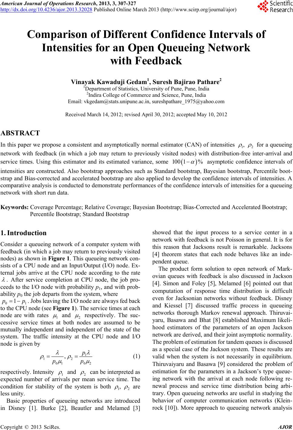
American Journal of Operations Research, 2013, 3, 307-327
http://dx.doi.org/10.4236/ajor.2013.32028 Published Online March 2013 (http://www.scirp.org/journal/ajor)
Comparison of Different Confidence Intervals of
Intensities for an Open Queueing Network
with Feedback
Vinayak Kawaduji Gedam1, Suresh Bajirao Pathare2
1Department of Statisti cs, University of Pune, Pune, India
2Indira College of Commerce and Science, Pune, India
Received March 14, 2012; revised April 30, 2012; accepted May 10, 2012
ABSTRACT
In this paper we propose a consistent and asymptotically no rmal estimator (CAN) of intensities 1

, 2

for a queueing
network with feedback (in which a job may return to previously visited nodes) with distribution-free inter-arrival and
service times. Using this estimator and its estimated variance, some


100 1%   asymptotic confidence intervals of
intensities are constructed. Also bootstrap approaches such as Standard bootstrap, Bayesian bootstrap, Percentile boot-
strap and Bias-corrected and accelerated bootstrap are also applied to develop the confidence intervals of intensities. A
comparative analysis is conducted to demonstrate perfo rmances of the confidence intervals of intensities for a queu eing
network with short run data.
Keywords: Coverage Percentage; Relative Coverage; Bayesian Bootstrap; Bias-Corrected and Accelerated Bootstrap;
Percentile Bootstrap; Standard Bootstrap
1. Introduction
Consider a queueing network of a computer system with
feedback (in which a job may return to previously visited
nodes) as shown in Figure 1. This queueing network con-
sists of a CPU node and an Input/Output (I/O) node. Ex-
ternal jobs arrive at the CPU node according to the rate

. After service completion at CPU node, the job pro-
ceeds to the I/O node with probability p1, and with prob-
ability p0 the job depart s f rom the system, where
01
1pp . Jobs lea ving the I/ O node are always fe d back
to the CPU node (see Figure 1). The service tim es at each
node are with rates 1

and 2

respectively. The suc-
cessive service times at both nodes are assumed to be
mutually independent and independent of the state of the
system. The traffic intensity at the CPU node and I/O
node is given by
1
12
01 02
,p
pp






(1)
respectively. Intensity 1

and 2

can be interpreted as
expected number of arrivals per mean service time. The
condition for stability of the system is both 1

, 2

are
less unity.
Basic properties of queueing networks are introduced
in Disney [1]. Burke [2], Beautler and Melamed [3]
showed that the input process to a service center in a
network with feedback is not Poisson in general. It is for
this reason that Jacksons result is remarkable. Jacksons
[4] theorem states that each node behaves like an inde-
pendent queue.
The product form solution to open network of Mark-
ovian queues with feedback is also discussed in Jackson
[4]. Simon and Foley [5], Melamed [6] pointed out that
computation of response time distribution is difficult
even for Jacksonian networks without feedback. Disney
and Kiessel [7] discussed traffic process in queueing
networks thorough Markov renewal approach. Thiruvai-
yaru, Basawa and Bhat [8] established Maximum likeli-
hood estimators of the parameters of an open Jackson
network a re derived, and t hei r j oi nt asy mptotic no rmality.
The probl em of estim ation fo r ta ndem q ueue s is disc ussed
as a special case of the Jackson system. These results are
valid when the system is not necessarily in equilibrium.
Thiruvaiyaru and Basawa [9] considered the problem of
estimation for the parameters in a Jackson’s type queue-
ing network with the arrival at each node following re-
newal process and service time distribution being arbi-
trary. Open queu eing networks are usefu l in studying the
behavior of computer communication networks (Klein-
rock [10]). More approach to queueing network analysis

V. K. GEDAM, S. B. PATHARE
308
Figure 1. An open queueing ne twork with feedback.
developed by Buzen and Denning [11]. Efron [12-14] the
greatest statistician in the field of nonparametric resam-
pling approach, originally developed and proposed the
bootstrap, which is a resampling technique that can be
effectively applied to estimate the sampling distribution
of any statistic. Sp ecifically, one can utilize the bootstrap
method to approximate the sampling distribution of a
statistic defined by a random sample from a population
with unknown probability distribution. And due to the
popularity of PC and statistical software, today the boot-
strap becomes the most powerful nonparametric estima-
tion procedure. Based upon the bootstrap resampling
technique, most statisticians utilize the standard bootstrap
(SB), percentile bootstrap (PB), and bias-corrected and
accelerated bootstrap (BCaB) approaches to produce
confidence intervals for practical problems.
Besides the standard bootstrap (SB) technique, Rubin
[15] presented the Bayesian bootstrap (BB) technique of
resampling. Miller [16] showed that the SB can be re-
garded as an extension of the jackknife. The BB is a
natural Bayesian analogue of the SB. The BB simulates
the posterior distribution of parameters under particular
model specifications, whereas the SB simulates the esti-
mated sampling distribution of a statistic estimating the
parameters. Both SB and BB can be applied to construct
confidence intervals of intensity for a queueing system
with distribution-free inter-arrival and service times.
Chu and Ke [17] constructed new confidence intervals
of mean response time for an M/G/1 FCFS queueing
system. Also, they performed the accuracy of bootstrap
confidence intervals through calculating the coverage
probability and the average length of confidence intervals.
Chu and Ke [18] proposed a consistent and asymptoti-
cally normal (CAN) estimator of the mean response time
for a G/M/1 queueing system, which is based on the
fixed point of empirical Laplace function. Ke and Chu
[19] proposed a consistent and asymptotically normal
estimator of intensity for a queueing system with distri-
bution-free interarrival and service times. Also, they
computed confidence intervals, testing statistical hy-
pothesi s of int ensi ty and powe r funct ion as soci ated wit h it
in this paper. Ke and Chu [20] constructed new confi-
dence intervals of intensity for a queueing system, which
are based on different bootstrap methods. They also per-
formed the accuracy of these bootstrap confidence inter-
vals through calcu lating the coverage probability and the
expected length of confidence intervals. They first pro-
posed bootstrapping technique and concept of relative
coverage to queueing system. They studied five estima-
tion approaches of intensity for a queueing system with
distribution free inter-arrival and service times for short
run. They have introduced a new measure called relative
coverage to assess the efficient performances of confi-
dence intervals.
In this paper we propose non parametric interval esti-
mation approach to intensities 1

, 2

for a open queue-
ing network with feedback. In Section 2 we prove that
the natural estimators 1
ˆ

, 2
ˆ

of intensities 1

and 2

are strongly consistent and asymptotically normal (CAN).
Based on the asymptotical normality of 1
ˆ

, 2 ˆ

, we can
construct a CAN confidence interval of 1

and 2

. Next
in Section 3 we establish the SB confidence interval of
1

, 2

via the standard bootstrap approach. In Section 4
we developed the derivation of the BB confidence inter-
val of 1

, 2

in terms of the Bayesian bootstrap ap-
proach. The percentile bootstrap (PB) confidence inter-
vals of 1

, 2

are developed in Section 5. In Section 6
we developed the bias-corrected and accelerated boot-
strap (BCaB) confidence intervals. A numerical simula-
tion study is conducted in Section 7 to demonstrate per-
formances of the interval estimation approaches for an
open queueing network with feedback using short run
data. All simulation results are shown by appropriate
tables for illustrating performances of the five interval
estimation approaches. Finally, we make some conclu-
sions in Section 8.
2. Nonparametric Statistical Inference of
Intensities
Let X1 and Y1 be nonnegative random variables repre-
sents the inter-arrival and service time at CPU node.
Similarly X2 and Y2 be nonnegative random variables
represents the inter-arrival and service time at I/O node
respectively. Given that a job just completed CPU node
burst, it will next request I/O node service with probability
1
p and with probability 0 p, where 01 1pp departs
from the system. The random variables at CPU node and
I/O node are independent. The intensities are defined as
follows:
1
1
0
1
Y
X
p

  and 2
2
0
21
Y
X
p
p



, (2)
where 1
X

, 2
X

denote the mean inter-arrival times at
CPU node and I/O node respectively. Similarly 1
Y

, 2
Y

denote the mean service times at CPU node and I/O node
respectively. Equation (2) is equivalent to Equation (1).
2.1. Estimating Intensities
Assume that 11 121 ,,,
n
X
XX is a random sample drawn

V. K. GEDAM, S. B. PATHARE
309
from X1 and 011 01201 ,,,
n
pY pYpY is a random sample
drawn from Y1. Let

101
,
ii
X
pY represents inter-arrival
time and service time for the ith customer of CPU node.
Similarly assume 121 12212
,,,
m
pX pXpX is a random
sample drawn from X2 and 021 02202
,,,
m
pY pYpY is a
random sample drawn from Y2. Let

12 02
,
ii
pXpY
represents inter-arrival time and service time for the ith
customer of I/O node.
Let 1212
,,,
X
XYY be the sample means of X1, X2, Y1,
Y2 respectively.
112 12
11
1012 02
11
11
,
11
,
nm
ii
ii
nm
ii
ii
X
XX pX
nm
YpYYpY
nm






According to the Strong Law of Large Numbers, we
know that 1212
,,,
X
XYY are strongly consistent estima-
tor of 1212 ,,,
XXYY


respectively. Thus a strongly
consistent estimator of intensities are given by
12
12
12
ˆˆ
,
YY
X
X
  (3)
In practical queueing network, the true distributions of
X1, X2, Y1, Y2 are rarely known, so the exact distributions
of 12
ˆˆ ,

 cannot be derived. But under the assumption
that X1 and Y1, X2 and Y2 being independent, the asymp-
totic distributions of 12
ˆˆ ,

 can be developed by the
following procedures.
Firstly, according to the Central Limit Theorem (see
[21] p. 234), w e have


11
11
2
1
2
10
0, and
0,
D
XX
D
YY
nX N
nY pN



 (4)
where 1
2
X

and 1
2
Y

are variances of X1 and Y1, respec-
tively.
Also,


22
22
2
21
2
20
0, and
0, ,
D
XX
D
YY
mX pN
mY pN



 (5)
where 2
2
X

and 2
2
Y

are variances of X2 and Y2, re-
spectively, and D

 denotes convergence in distribu-
tion.
Next note that


1
1
1111
1
11
0
1
1
100 1
1
ˆ
.
Y
X
XYYX
X
n
p
Y
nX
nYp pX
X







 



 


Also,



2
2
222 2
2
22
0
2
21
120021
12
ˆ
.
Y
X
XYY X
X
m
p
Y
mXp
mpY ppXp
pX







 




 



(6)
Therefore by the Slutsky’s theorem [see [21] p. 227],
we get



2
11 1
ˆ0,
D
nN

 ,
where 111 1
1
22 222
0
2
14
XY YX
X
p




.
And



2
22 2
ˆ0,
D
mN

  (7)
where 222 2
2
22222 2
10
2
224
1
XY YX
X
pp
p




.
Now, set
11
22
22 222
101
2
14
1
222222
12 02
2
224
12
ˆand
ˆ,
YX
YX
XS pYS
X
pXS pYS
pX






(8)
where
 
 
11
22
22
22
11 011
11
22
22
122022
11
11
,
11
and .
nn
XiY i
ii
mm
XiYi
ii
SXXSpYY
nn
SpXXSpYY
mm


 
 


Then 22
12
ˆˆ ,

 are strongly consistent estimators of
22
12
,

 respectively. Applying the Slutsky’s theorem
once again, we deduce that
 
 
11
1
22
2
ˆ0,1 and
ˆ
ˆ0,1
ˆ
D
D
nN
mN






(9)
Thus 12
ˆˆ
,

are strongly consistent and asymptoti-
cally normal (CAN) estimators with approximate vari-
ances 22
12
ˆˆ
,
nm


respectively.
2.2. Confidence Intervals
Using the CAN estimators 12
ˆˆ ,

and its associated
approximate variances 22
12
ˆˆ
,
nm


we construct a confi-

V. K. GEDAM, S. B. PATHARE
310
dence intervals of intensities 12
&

 for a open queue-
ing network with feedback. Let z

be the upper th

quantile of the standard normal distribution, by the as-
ymptotic distribution of




112 2
12
ˆˆ
&
ˆˆ
nm




in expression (9), an approximate

100 1%   confi-
dence interval of 12
&

 are obtained as

11
22
1
21 21
111
ˆ
1ˆ
ˆˆ
ˆˆ
n
Pz z
zz
Pnn









  



 


Consequently, an approximate


100 1%   confi-
dence interval of 1

is
21 21
11
ˆˆ
ˆˆ
,
zz
nn








. (10)
Similarly, an approximate


100 1%   confidence
interval of 2

is
22 22
22
ˆˆ
ˆˆ
,
zz
mm








. (11)
3. Standard Bootstrap Confidence Intervals
of Intensities
Now the bootstrap confidence intervals are developed as
follows:
Let 11 121
,,,
n
x
xx be a random sample of n observa-
tions taken from the population X1 and 011 012 ,,,pypy 
01n
py be a random sample of n observations taken from
the population Y1. According to the bootstrap procedure,
a simple random sample 11 121
,,,
n
x
xx


 can be taken
from the empirical distribution function of 11 121
,,,
n
x
xx
called a bootstrap sample from 11121
,,,
n
x
xx. Also, we
can draw a bootstrap sample 01101201
,,,
n
py pypy
 
 from
01101201
,,,
n
py pypy. It follows from Equation (2) that
an estimate of intensity 1

can be calculated from boot-
strap samples as
1
11
ˆy
x




, (12)
where 1
x
 and 1
y
 are the sample means of 11 12
,,,xx


1n
x
 and011 01201
,,,
n
py pypy
 
 respectively and 1
ˆ


is
called a bootstrap estimate of 1

. The above resampling
process can be repeated N1 times. The N1 bootstrap esti-
mates 1
11 121
ˆˆˆ
,,,
N


 
 can be computed from the boot-
strap resamples. Averaging the N1 bootstrap estimates we
obtain that
1
11
1
1
1
ˆˆ
N
N
i
i
N





(13)
is the bootstrap estimate of 1

. And the standard devia-
tion of 1
ˆ

can be estimated by
 
1
11
12
2
1
1
1
1
ˆˆˆ .
1
N
NiN
i
sd N 









 (14)
Because the central limit theorem implies that the dis-
tribution of 1
ˆ

is approximately nor mal. A


100 1%  
SB confidence interval for 1

is




11
12 12
ˆˆ ˆˆ
,,
NN
zsd zsd

  (15)
Similarly 121 12212
,,,
m
px pxpx is a random sample
of m observation drawn from population X2 and 021
,py
022 02
,, m py py is a sample of m observations taken
from the population 2
Y. According to the bootstrap pro-
cedure, a simple random sample 121 12212 ,,,
m
px pxpx
 

can be taken from the empirical distribution function of
121 12212
,,,
m
px pxpx called a bootstrap sample from
121 12212
,,,
m
px pxpx. Also, we can draw a bootstrap
sample 021 02202
,,,
m
py pypy


 from 021 022 ,,,pypy 
02m
py . An estimate of intensity 2

can be calculated
from bootstrap samples as
2
2
2
ˆy
x




, (16)
where 2
x

and 2
y

are the sample means of 121 ,px

122 12
,, m px px


 and 021 02202 ,,,
m
py pypy
 
 respec-
tively and 2
ˆ


is called a bootstrap estimate of 2

. The
above resampling process can be repeated M1 times. The
M1 bootstrap estimates 1
21 222
ˆˆˆ ,,,
M


 
 can be com-
puted from the bootstrap resamples. Averaging the M1
bootstrap estimates we obtain that
1
12
1
1
1
ˆˆ
M
M
i
i
M



 (17)
is the bootstrap estimate of 2

. And the standard devia-
tion of 2
ˆ

can be estimated by
 
11
12
2
2
1
1
1
ˆˆˆ .
1
M
MiM
i
sd M 









 (18)
Because the central limit theorem implies that the dis-
tribution of 2
ˆ

is approximately normal. A


100 1%  
SB confidence interval for 2

is




11
22 22
ˆˆˆˆ
,,
MM
zsd zsd

  (19)
4. Bayesian Bootstrap Confidence Intervals
of Intensities
The Bayesian bootstrap is analogous to the standard
bootstrap. Each BB replication generates a posterior
probability for each 1i
x
. Specifically, one BB replicatio n
is generated by drawing 1n uniform

0,1 random
numbers 12 1
,, ,
n
rr r

, ordering them, and calculating the
gaps
 
11 iii
wrr


, 1, 2,,in

, where

00r

and

V. K. GEDAM, S. B. PATHARE
311

1
n
r. Then

111121
,,,
in
www w is the vector of
probabilities attached to the inter-arrival data values
11 121
,,,
n
x
xx in that BB replicatio n . Considering all BB
replications gives the BB distribution of the distribution
of X1 and thus of any parameter of this distribution.
Hence fo r 1
X

(the mean of X1), in each BB replication
we calculate 1
X

as if 1i w were the probability that
1i
X
x that is, we calculate 111
1
n
ii
i
x
wx


. The dis-
tribution of the values of 1
x
 overall BB replications is
the BB distribution of 1
X

.
Also, generating a vector of probabilities

11112 1
,,,
n
vvv v attached to the service time data
values 011 01201
,,,
n
py pypy in a BB replication, and we
calculate 1011
1
n
ii
i
ypvy


 for 1
Y

(the mean of Y1).
Then in terms of equation (2) an estimate of intensity 1

can be calculated from BB replications as
1
11
ˆy
x






, (20)
where 1
ˆ

 is called a Bayesian bootstrap estimate of
1

. The above BB process can be repeated N1 times. The
N1 BB estimates, 1
11 121
ˆˆˆ ,,,
N


 
 can be computed
from the BB replications. Averag ing the N1 BB estimates,
we obtain that
1
1
1
1
1
ˆˆ
N
B
Bj
j
N






, (21)
is the BB estimate of 1

. And the standard deviation of
1
ˆ

can be estimated by


1
1
2
2
1BB
1
1
1
ˆˆˆ
1
N
BB j
j
sd N 








. (22)
Applying the asymptotical normality of 1
ˆ

, a

100 1%   BB confidence interval for 1

is
 

12 12
ˆˆˆˆ
,
BB BB
zsd zsd



 . (23)
Similarly each BB replication generates a posterior
probability for each 2i
x
. Specifically, one BB replica-
tion is generated by drawing 1m uniform

0,1 ran-
dom numbers 121
,, ,
m
rr r

, ordering them and calculat-
ing the gaps
 
21,1,2,, iii
wrrim

 , where

00r

and

1
m
r. Then

221222
,,,
im
www w is the vec-
tor of probabilities attached to the inter-arrival data val-
ues 121 12212 ,,,
m
px pxpx in that BB replication. Con-
sidering all BB replications gives the BB distribution of
the distribution of X2 and thus of any parameter of this
distribution. Hence for 2
X

(the mean of X2), in each
BB replication we calculate 2
X

as if 2i w were the
probability that 22i
X
x that is, we calculate
2122
1
m
ii
i
x
pwx


. The distribution of the values of 2
x


over all BB replications is the BB distribution of 2
X

.
Also, generating a vector of probabilities


22122 2
,,,
m
vvv v attached to the service time data
values 021 02202
,,,
m
py pypy in a BB replication, and
we calculate 2022
1
m
ii
i
y
pvy


 for 2
Y

(the mean of Y2).
Then in terms of Equation (2) an estimate of intensity
2

can be calculated from BB replications as
2
22
ˆy
x




, (24)
where 2
ˆ


 is called a Bayesian bootstrap estimate of
2

. The above BB process can be repeated M1 times.
The M1 BB estimates, 1
21 222
ˆˆˆ
,,,
M



 can be com-
puted from the BB replications. Averaging the M1 BB
estimates, we obtain that
1
2
1
1
1
ˆˆ
M
B
Bj
j
M




 , (25)
is the BB estimate of 2

. And the standard deviation of
2
ˆ

can be estimated by


12
2
1
1
1
ˆˆ ˆ
1
M
BBj BB
j
sd M 




 





. (26)
Applying the asymptotical normality of 2
ˆ

, a


100 1%   BB confidence interval for 2

is




22 22
ˆˆˆ ˆ
,
BB BB
zsd zsd




 (27)
5. Percentile Bootstrap Confidence Intervals
of Intensities
Let 1
11 121
ˆˆˆ
,,,
N




 and 1
21 222
ˆˆˆ
,,,
M


 
 call the boot-
strap distribution of 12
ˆˆ
,

 respectively. Let


1
ˆ1

,




111
ˆˆ 2, ,N 

 and
 


22 21
ˆˆˆ 1,2, ,
M
 
 
 be
order statistics of 1
11 121
ˆˆ ˆ
,,,
N
 


 and 1
21 222
ˆˆˆ
,,,
M




respectively. Then utilizing the

1002 th  and


100 12th   percentage points of the bootstrap dis-
tribution, a


100 1%   PB confidence interval for 1

,
2

are obtained as
11 11
ˆˆ
,1,
22
NN




 

 
 


 
 

 

 

 
 

(28)
21 21
ˆˆ
,1,
22
MM




 

 
 


 
 

 

 

 
 

(29)
where [x] denotes the greatest integer less than or equal
to x.
6. Bias-Corrected and Accelerated Boo tstr ap
Confidence Intervals of Intensities
The bootstrap distribution 1
11 121
ˆˆ ˆ
,,,
N
 
 
 and 21
ˆ,



V. K. GEDAM, S. B. PATHARE
312
1
22 2
ˆˆ
,,
M



 may be biased. This method is designed to
correct this potential bias of the bootstrap designed. Set

111
11
ˆˆ
Nj
j
I
pN




 and

122
11
ˆˆ
Mj
j
I
pM




 ,
where

I
 is the indicator function. Define


1
0
ˆ
zp 



and

1
1
ˆ
zp 

, where 1

 denotes the inverse func-
tion of the standard normal distribution

. Except for
correcting the potential bias of the bootstrap distribution,
we can accelerate convergence of bootstrap distribution.
Let

1
X
i
 and

01
pY i
 denote the original samples
with the ith observation x1i and 01i py deleted, also let
1
ˆi

b e the estimator of 1

calculated by using


1
X
i

and

01
pY i
 Define 11
1
1ˆ
n
i
i
n





, Similarly


12
pXi
,

02
pY i
 denote the original samples with the ith obser-
vation 12i px and 02i py deleted, also 2
ˆi

be the esti-
mator of 2

calculated by using

12
pX i
 and


02
pY i
.
Define 22
1
1ˆ
m
i
i
m





And






3
2
3
2
3
11
1
1
2
11
1
3
22
1
2
2
22
1
ˆ
ˆ,
ˆ
6
ˆ
ˆ
ˆ
6
n
i
i
n
i
i
m
i
i
m
i
i
a
a










 








 














(30)
where 011
ˆ ˆˆ
,,zza , and 2
ˆ
a are named bias-correction and
acceleration respectively.
Thus a

100 1%   Bias-corrected and accelerated
bootstrap (BCaB) Confidence Interval of intensities 1

,
2

are constructed by




 
111112
ˆˆ
,NN 

(31)







213 214
ˆˆ
,MM 

(32)
where


02
10
102
ˆ
ˆˆˆ
1
zz
zaz z













02
20
102
ˆ
ˆˆˆ
1
zz
zaz z













12
31
21 2
ˆ
ˆˆˆ
1
zz
zaz z

















12
41
21 2
ˆ
ˆˆˆ
1
zz
zazz















7. Simulation Study
To evaluate performances of the different interval esti-
mation approaches mentioned above for an open queue-
ing network with feedback using short run data, a nu-
merical simulation study was undertaken. Most of the
statisticians assess performances of interval estimations
in terms of coverage percentages or average lengths of
confidence intervals. However, through simulation study
in the research work, we find that larger coverage per-
centages of confidence interval may often be due to
wider standard deviation of interval estimation methods.
Moreover, narrower confidence intervals may often lead
to smaller coverage percentages. Hence, both coverage
percentage and average length are not efficient for ap-
praising interval estimation methods. In order to over-
come above two shortcomings, we propose a measure
called relative coverage to evaluate performances of in-
terval estimation methods where,
Coveragepercentage
Relative coverageAv eragelength .
The larger of the relative coverage implies the better
performance of the corresponding con fidence interval. In
order to reach this goal, we set a continuous distribution
with mean 1

on inter-arrival time X1 and X2. Also set
continuous distribution with mean 1 1

on the service
time Y1 at CPU node and continuous distribution with
mean 2 1

on the service time Y2 at I/O node. The lev-
els of p0 considered in the simulation study are 0.1 to 0.9
where as levels of p1 are 0.9 to 0.1, where p0 is the prob-
ability that the job departs from the system and p1 is the
probability that after service completion at CPU node, the
job proceeds to the I/O node. This means with probability
00.1p

the job departs from the system and with
probability 10.9p

, after service completion at CPU
node, the job proceeds to the I/O node and so on. Also we
have considered the values of 1

and 2

such that
11


and 21


for simulation study. Note that in
Table 1 wherever 11

 and 21

 such values of
1

and 2

are not considered for simulation study.
The intensity parameters 1

and 2

are calculated
using Equation (1). The different values of

, 1
µ
, 2
µ
,
p0 and p1 are considered for simulation study as shown in
Table 1.
For different levels of 1

, random samples of inter-
arrival times 11 121 ,,,
n
X
XX and service times 011 pY ,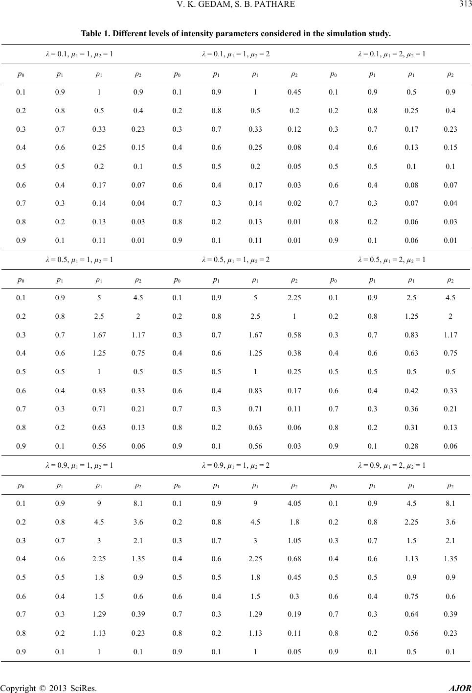

V. K. GEDAM, S. B. PATHARE
313
Table 1. Different levels of intensity parameters considered in the simulation study.
λ = 0.1, µ1 = 1, µ2 = 1 λ = 0.1, µ1 = 1, µ2 = 2 λ = 0.1, µ1 = 2, µ2 = 1
p0 p1 ρ1 ρ2 p0 p1 ρ1 ρ2 p0 p1 ρ1 ρ2
0.1 0.9 1 0.9 0.1 0.9 1 0.45 0.1 0.9 0.5 0.9
0.2 0.8 0.5 0.4 0.2 0.8 0.5 0.2 0.2 0.8 0.25 0.4
0.3 0.7 0.33 0.23 0.3 0.7 0.33 0.12 0.3 0.7 0.17 0.23
0.4 0.6 0.25 0.15 0.4 0.6 0.25 0.08 0.4 0.6 0.13 0.15
0.5 0.5 0.2 0.1 0.5 0.5 0.2 0.05 0.5 0.5 0.1 0.1
0.6 0.4 0.17 0.07 0.6 0.4 0.17 0.03 0.6 0.4 0.08 0.07
0.7 0.3 0.14 0.04 0.7 0.3 0.14 0.02 0.7 0.3 0.07 0.04
0.8 0.2 0.13 0.03 0.8 0.2 0.13 0.01 0.8 0.2 0.06 0.03
0.9 0.1 0.11 0.01 0.9 0.1 0.11 0.01 0.9 0.1 0.06 0.01
λ = 0.5, µ1 = 1, µ2 = 1 λ = 0.5, µ1 = 1, µ2 = 2 λ = 0.5, µ1 = 2, µ2 = 1
p0 p1 ρ1 ρ2 p0 p1 ρ1 ρ2 p0 p1 ρ1 ρ2
0.1 0.9 5 4.5 0.1 0.9 5 2.25 0.1 0.9 2.5 4.5
0.2 0.8 2.5 2 0.2 0.8 2.5 1 0.2 0.8 1.25 2
0.3 0.7 1.67 1.17 0.3 0.7 1.67 0.58 0.3 0.7 0.83 1.17
0.4 0.6 1.25 0.75 0.4 0.6 1.25 0.38 0.4 0.6 0.63 0.75
0.5 0.5 1 0.5 0.5 0.5 1 0.25 0.5 0.5 0.5 0.5
0.6 0.4 0.83 0.33 0.6 0.4 0.83 0.17 0.6 0.4 0.42 0.33
0.7 0.3 0.71 0.21 0.7 0.3 0.71 0.11 0.7 0.3 0.36 0.21
0.8 0.2 0.63 0.13 0.8 0.2 0.63 0.06 0.8 0.2 0.31 0.13
0.9 0.1 0.56 0.06 0.9 0.1 0.56 0.03 0.9 0.1 0.28 0.06
λ = 0.9, µ1 = 1, µ2 = 1 λ = 0.9, µ1 = 1, µ2 = 2 λ = 0.9, µ1 = 2, µ2 = 1
p0 p1 ρ1 ρ2 p0 p1 ρ1 ρ2 p0 p1 ρ1 ρ2
0.1 0.9 9 8.1 0.1 0.9 9 4.05 0.1 0.9 4.5 8.1
0.2 0.8 4.5 3.6 0.2 0.8 4.5 1.8 0.2 0.8 2.25 3.6
0.3 0.7 3 2.1 0.3 0.7 3 1.05 0.3 0.7 1.5 2.1
0.4 0.6 2.25 1.35 0.4 0.6 2.25 0.68 0.4 0.6 1.13 1.35
0.5 0.5 1.8 0.9 0.5 0.5 1.8 0.45 0.5 0.5 0.9 0.9
0.6 0.4 1.5 0.6 0.6 0.4 1.5 0.3 0.6 0.4 0.75 0.6
0.7 0.3 1.29 0.39 0.7 0.3 1.29 0.19 0.7 0.3 0.64 0.39
0.8 0.2 1.13 0.23 0.8 0.2 1.13 0.11 0.8 0.2 0.56 0.23
0.9 0.1 1 0.1 0.9 0.1 1 0.05 0.9 0.1 0.5 0.1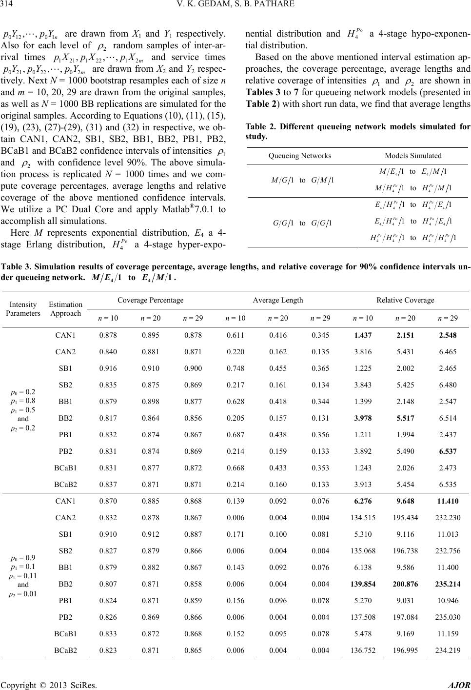

V. K. GEDAM, S. B. PATHARE
314
012 01
,, n pY pY are drawn from X1 and Y1 respectively.
Also for each level of 2

random samples of inter-ar-
rival times 121 12212 ,,,
m
pX pXpX and service times
021 02202
,,,
m
pY pYpY are drawn from X2 and Y2 respec-
tively. Next N = 1000 bootstrap r esamples each of size n
and m = 10, 20, 29 are drawn from the original samples,
as well as N = 1000 BB replications are simulated for the
original samples. According to Equations (10), (11), (15),
(19), (23), (27)-(29), (31) and (32) in respective, we ob-
tain CAN1, CAN2, SB1, SB2, BB1, BB2, PB1, PB2,
BCaB1 and BCaB2 confidence intervals of intensities 1

and 2

with confidence level 90%. The above simula-
tion process is replicated N = 1000 times and we com-
pute coverage percentages, average lengths and relative
coverage of the above mentioned confidence intervals.
We utilize a PC Dual Core and apply Matlab®7.0.1 to
accomplish all simulations.
Here M represents exponential distribution, E4 a 4-
stage Erlang distribution, 4
P
e
H
a 4-stage hyper-expo-
nential distribution and 4
P
o
H
a 4-stage hypo-exponen-
tial distribution.
Based on the above mentioned interval estimation ap-
proaches, the coverage percentage, average lengths and
relative coverage of intensities 1

and 2

are shown in
Tables 3 to 7 for queueing network models (presented in
Table 2) with short run data, we find that average lengths
Table 2. Different queueing network models simulated for
study.
Queueing Networks Models Simulated
41
M
E to 41EM
1
M
G to 1GM
41
Pe
MH to 41
Pe
H
M
44
1
Pe
EH to 44 1
Pe
H
E
44
1
Po
EH to 44 1
Po
H
E
1GG to 1GG
44
1
Pe Po
HH to 44 1
Po Pe
HH
Table 3. Simulation results of coverage percentage, average lengths, and relative coverage for 90% confidence intervals un-
der queueing network. 41ME to 41EM .
Coverage Percentage Average Length Relative Coverage
Intensity
Parameters Estimation Approach n = 10 n = 20 n = 29 n = 10 n = 20 n = 29 n = 10 n = 20 n = 29
CAN1 0.878 0.895 0.878 0.611 0.416 0.345 1.437 2.151 2.548
CAN2 0.840 0.881 0.871 0.220 0.162 0.135 3.816 5.431 6.465
SB1 0.916 0.910 0.900 0.748 0.455 0.365 1.225 2.002 2.465
SB2 0.835 0.875 0.869 0.217 0.161 0.134 3.843 5.425 6.480
BB1 0.879 0.898 0.877 0.628 0.418 0.344 1.399 2.148 2.547
BB2 0.817 0.864 0.856 0.205 0.157 0.131 3.978 5.517 6.514
PB1 0.832 0.874 0.867 0.687 0.438 0.356 1.211 1.994 2.437
PB2 0.831 0.874 0.869 0.214 0.159 0.133 3.892 5.490 6.537
BCaB1 0.831 0.877 0.872 0.668 0.433 0.353 1.243 2.026 2.473
p0 = 0.2
p1 = 0.8
ρ1 = 0.5
and
ρ2 = 0.2
BCaB2 0.837 0.871 0.871 0.214 0.160 0.133 3.913 5.454 6.535
CAN1 0.870 0.885 0.868 0.139 0.092 0.076 6.276 9.648 11.410
CAN2 0.832 0.878 0.867 0.006 0.004 0.004 134.515 195.434 232.230
SB1 0.910 0.912 0.887 0.171 0.100 0.081 5.310 9.116 11.013
SB2 0.827 0.879 0.866 0.006 0.004 0.004 135.068 196.738 232.756
BB1 0.879 0.882 0.867 0.143 0.092 0.076 6.138 9.586 11.400
BB2 0.807 0.871 0.858 0.006 0.004 0.004 139.854 200.876 235.214
PB1 0.824 0.871 0.859 0.156 0.096 0.078 5.270 9.031 10.946
PB2 0.826 0.869 0.866 0.006 0.004 0.004 137.508 197.084 235.030
BCaB1 0.833 0.872 0.868 0.152 0.095 0.078 5.478 9.169 11.159
p0 = 0.9
p1 = 0.1
ρ1 = 0.11
and
ρ2 = 0.01
BCaB2 0.823 0.871 0.865 0.006 0.004 0.004 136.752 196.995 234.219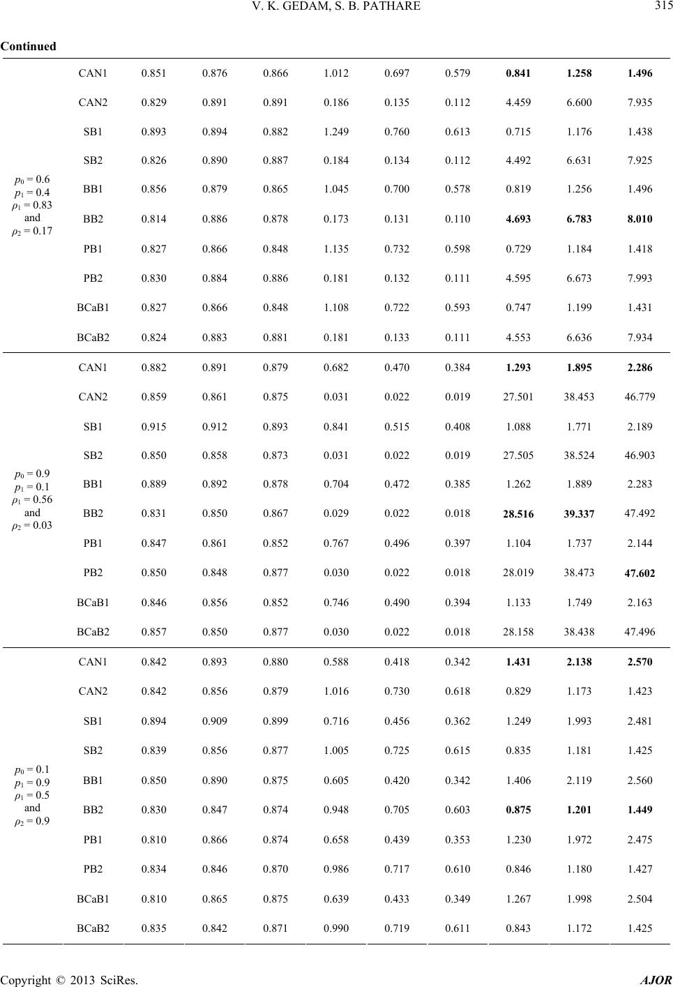

V. K. GEDAM, S. B. PATHARE
315
Continued
CAN1 0.851 0.876 0.866 1.012 0.697 0.579 0.841 1.258 1.496
CAN2 0.829 0.891 0.891 0.186 0.135 0.112 4.459 6.600 7.935
SB1 0.893 0.894 0.882 1.249 0.760 0.613 0.715 1.176 1.438
SB2 0.826 0.890 0.887 0.184 0.134 0.112 4.492 6.631 7.925
BB1 0.856 0.879 0.865 1.045 0.700 0.578 0.819 1.256 1.496
BB2 0.814 0.886 0.878 0.173 0.131 0.110 4.693 6.783 8.010
PB1 0.827 0.866 0.848 1.135 0.732 0.598 0.729 1.184 1.418
PB2 0.830 0.884 0.886 0.181 0.132 0.111 4.595 6.673 7.993
BCaB1 0.827 0.866 0.848 1.108 0.722 0.593 0.747 1.199 1.431
p0 = 0.6
p1 = 0.4
ρ1 = 0.83
and
ρ2 = 0.17
BCaB2 0.824 0.883 0.881 0.181 0.133 0.111 4.553 6.636 7.934
CAN1 0.882 0.891 0.879 0.682 0.470 0.384 1.293 1.895 2.286
CAN2 0.859 0.861 0.875 0.031 0.022 0.019 27.501 38.453 46.779
SB1 0.915 0.912 0.893 0.841 0.515 0.408 1.088 1.771 2.189
SB2 0.850 0.858 0.873 0.031 0.022 0.019 27.505 38.524 46.903
BB1 0.889 0.892 0.878 0.704 0.472 0.385 1.262 1.889 2.283
BB2 0.831 0.850 0.867 0.029 0.022 0.018
28.516 39.337 47.492
PB1 0.847 0.861 0.852 0.767 0.496 0.397 1.104 1.737 2.144
PB2 0.850 0.848 0.877 0.030 0.022 0.018 28.019 38.473 47.602
BCaB1 0.846 0.856 0.852 0.746 0.490 0.394 1.133 1.749 2.163
p0 = 0.9
p1 = 0.1
ρ1 = 0.56
and
ρ2 = 0.03
BCaB2 0.857 0.850 0.877 0.030 0.022 0.018 28.158 38.438 47.496
CAN1 0.842 0.893 0.880 0.588 0.418 0.342 1.431 2.138 2.570
CAN2 0.842 0.856 0.879 1.016 0.730 0.618 0.829 1.173 1.423
SB1 0.894 0.909 0.899 0.716 0.456 0.362 1.249 1.993 2.481
SB2 0.839 0.856 0.877 1.005 0.725 0.615 0.835 1.181 1.425
BB1 0.850 0.890 0.875 0.605 0.420 0.342 1.406 2.119 2.560
BB2 0.830 0.847 0.874 0.948 0.705 0.603 0.875 1.201 1.449
PB1 0.810 0.866 0.874 0.658 0.439 0.353 1.230 1.972 2.475
PB2 0.834 0.846 0.870 0.986 0.717 0.610 0.846 1.180 1.427
BCaB1 0.810 0.865 0.875 0.639 0.433 0.349 1.267 1.998 2.504
p0 = 0.1
p1 = 0.9
ρ1 = 0.5
and
ρ2 = 0.9
BCaB2 0.835 0.842 0.871 0.990 0.719 0.611 0.843 1.172 1.425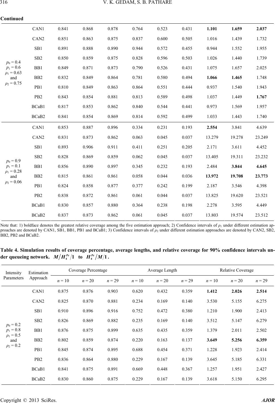

V. K. GEDAM, S. B. PATHARE
316
Continued
CAN1 0.841 0.868 0.878 0.764 0.523 0.431 1.101 1.659 2.037
CAN2 0.851 0.863 0.875 0.837 0.600 0.505 1.016 1.439 1.732
SB1 0.891 0.888 0.890 0.944 0.572 0.455 0.944 1.552 1.955
SB2 0.850 0.859 0.875 0.828 0.596 0.503 1.026 1.440 1.739
BB1 0.849 0.871 0.873 0.790 0.526 0.431 1.075 1.657 2.025
BB2 0.832 0.849 0.864 0.781 0.580 0.494 1.066 1.465 1.748
PB1 0.810 0.849 0.863 0.864 0.551 0.444 0.937 1.540 1.943
PB2 0.843 0.854 0.881 0.813 0.589 0.498 1.037 1.449 1.767
BCaB1 0.817 0.853 0.862 0.840 0.544 0.441 0.973 1.569 1.957
p0 = 0.4
p1 = 0.6
ρ1 = 0.63
and
ρ2 = 0.75
BCaB2 0.841 0.854 0.869 0.814 0.592 0.499 1.033 1.443 1.740
CAN1 0.853 0.887 0.896 0.334 0.231 0.193 2.554 3.841 4.639
CAN2 0.831 0.873 0.862 0.063 0.045 0.037 13.279 19.278 23.249
SB1 0.893 0.906 0.911 0.411 0.251 0.205 2.171 3.611 4.452
SB2 0.828 0.869 0.859 0.062 0.045 0.037 13.405 19.311 23.232
BB1 0.856 0.890 0.897 0.345 0.232 0.193 2.484 3.844 4.645
BB2 0.815 0.861 0.861 0.058 0.044 0.036
13.972 19.708 23.773
PB1 0.824 0.858 0.877 0.377 0.242 0.199 2.187 3.546 4.398
PB2 0.838 0.872 0.861 0.061 0.044 0.037 13.825 19.620 23.521
BCaB1 0.830 0.857 0.880 0.364 0.238 0.198 2.278 3.595 4.449
p0 = 0.9
p1 = 0.1
ρ1 = 0.28
and
ρ2 = 0.06
BCaB2 0.837 0.873 0.862 0.061 0.045 0.037 13.803 19.574 23.512
Note that: 1) boldface denotes the greatest relative coverage among the five estimation approach; 2) Confidence intervals of ρ1 under different estimation ap-
proaches are denoted by CAN1, SB1, BB1, PB1 and BCaB1; 3) Confidence intervals of ρ2 under different estimation approaches are denoted by CAN2, SB2,
BB2, PB2 and BCaB2.
Table 4. Simulation results of coverage percentage, average lengths, and relative coverage for 90% confidence intervals un-
der queueing network. 41
Pe
MH to 41
Pe
HM.
Coverage Percentage Average Length Relative Coverage
Intensity
Parameters Estimation Approach n = 10 n = 20 n = 29 n = 10 n = 20 n = 29 n = 10 n = 20 n = 29
CAN1 0.875 0.876 0.903 0.620 0.432 0.359 1.412 2.026 2.514
CAN2 0.825 0.870 0.881 0.234 0.169 0.140 3.530 5.155 6.275
SB1 0.910 0.896 0.916 0.752 0.472 0.380 1.210 1.900 2.413
SB2 0.826 0.869 0.882 0.235 0.169 0.140 3.512 5.147 6.279
BB1 0.876 0.875 0.899 0.635 0.435 0.359 1.379 2.011 2.502
BB2 0.802 0.859 0.874 0.220 0.163 0.137 3.649 5.256 6.359
PB1 0.845 0.874 0.895 0.688 0.454 0.371 1.228 1.923 2.414
PB2 0.836 0.864 0.880 0.229 0.167 0.139 3.645 5.185 6.331
BCaB1 0.841 0.875 0.891 0.669 0.448 0.367 1.257 1.951 2.427
p0 = 0.2
p1 = 0.8
ρ1 = 0.5
and
ρ2 = 0.2
BCaB2 0.830 0.860 0.875 0.229 0.167 0.139 3.618 5.150 6.295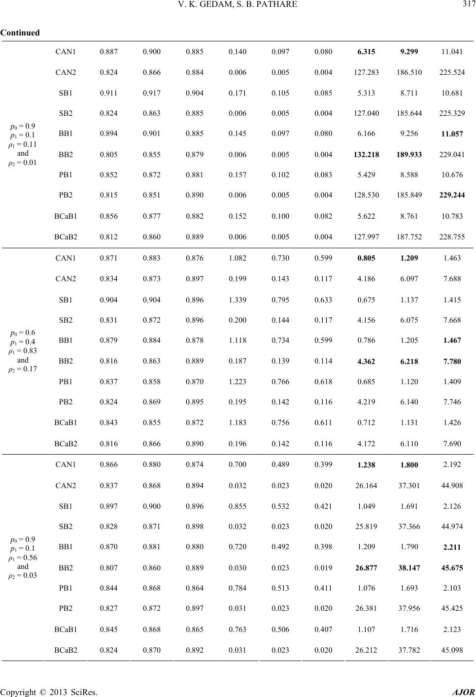

V. K. GEDAM, S. B. PATHARE
317
Continued
CAN1 0.887 0.900 0.885 0.140 0.097 0.080 6.315 9.299 11.041
CAN2 0.824 0.866 0.884 0.006 0.005 0.004 127.283 186.510 225.524
SB1 0.911 0.917 0.904 0.171 0.105 0.085 5.313 8.711 10.681
SB2 0.824 0.863 0.885 0.006 0.005 0.004 127.040 185.644 225.329
BB1 0.894 0.901 0.885 0.145 0.097 0.080 6.166 9.256 11.057
BB2 0.805 0.855 0.879 0.006 0.005 0.004
132.218 189.933 229.041
PB1 0.852 0.872 0.881 0.157 0.102 0.083 5.429 8.588 10.676
PB2 0.815 0.851 0.890 0.006 0.005 0.004 128.530 185.849 229.244
BCaB1 0.856 0.877 0.882 0.152 0.100 0.082 5.622 8.761 10.783
p0 = 0.9
p1 = 0.1
ρ1 = 0.11
and
ρ2 = 0.01
BCaB2 0.812 0.860 0.889 0.006 0.005 0.004 127.997 187.752 228.755
CAN1 0.871 0.883 0.876 1.082 0.730 0.599 0.805 1.209 1.463
CAN2 0.834 0.873 0.897 0.199 0.143 0.117 4.186 6.097 7.688
SB1 0.904 0.904 0.896 1.339 0.795 0.633 0.675 1.137 1.415
SB2 0.831 0.872 0.896 0.200 0.144 0.117 4.156 6.075 7.668
BB1 0.879 0.884 0.878 1.118 0.734 0.599 0.786 1.205 1.467
BB2 0.816 0.863 0.889 0.187 0.139 0.114 4.362 6.218 7.780
PB1 0.837 0.858 0.870 1.223 0.766 0.618 0.685 1.120 1.409
PB2 0.824 0.869 0.895 0.195 0.142 0.116 4.219 6.140 7.746
BCaB1 0.843 0.855 0.872 1.183 0.756 0.611 0.712 1.131 1.426
p0 = 0.6
p1 = 0.4
ρ1 = 0.83
and
ρ2 = 0.17
BCaB2 0.816 0.866 0.890 0.196 0.142 0.116 4.172 6.110 7.690
CAN1 0.866 0.880 0.874 0.700 0.489 0.399 1.238 1.800 2.192
CAN2 0.837 0.868 0.894 0.032 0.023 0.020 26.164 37.301 44.908
SB1 0.897 0.900 0.896 0.855 0.532 0.421 1.049 1.691 2.126
SB2 0.828 0.871 0.898 0.032 0.023 0.020 25.819 37.366 44.974
BB1 0.870 0.881 0.880 0.720 0.492 0.398 1.209 1.790 2.211
BB2 0.807 0.860 0.889 0.030 0.023 0.019 26.877 38.147 45.675
PB1 0.844 0.868 0.864 0.784 0.513 0.411 1.076 1.693 2.103
PB2 0.827 0.872 0.897 0.031 0.023 0.020 26.381 37.956 45.425
BCaB1 0.845 0.868 0.865 0.763 0.506 0.407 1.107 1.716 2.123
p0 = 0.9
p1 = 0.1
ρ1 = 0.56
and
ρ2 = 0.03
BCaB2 0.824 0.870 0.892 0.031 0.023 0.020 26.212 37.782 45.098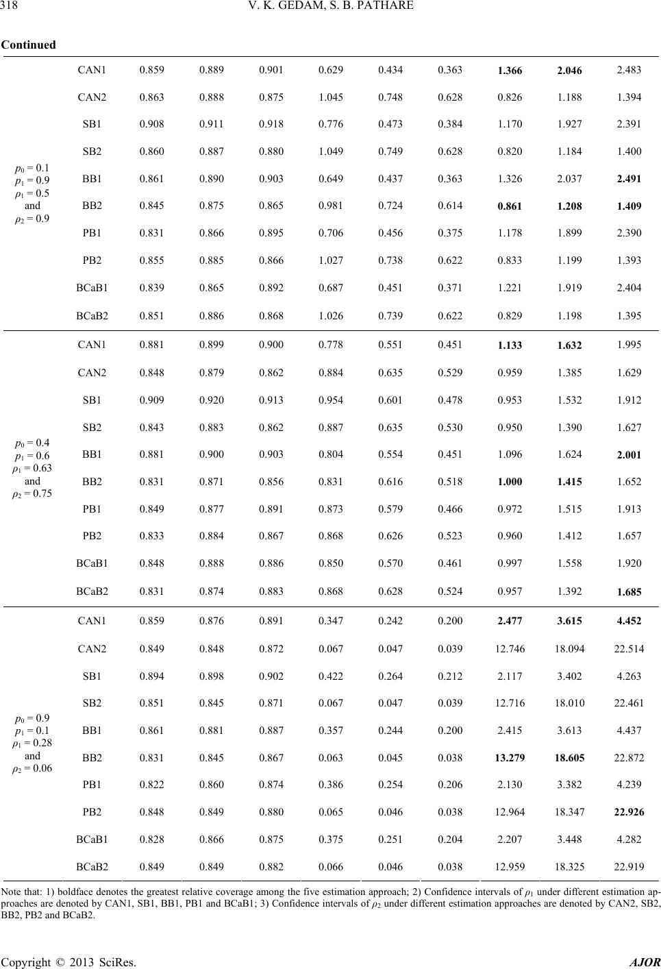

V. K. GEDAM, S. B. PATHARE
318
Continued
CAN1 0.859 0.889 0.901 0.629 0.434 0.363 1.366 2.046 2.483
CAN2 0.863 0.888 0.875 1.045 0.748 0.628 0.826 1.188 1.394
SB1 0.908 0.911 0.918 0.776 0.473 0.384 1.170 1.927 2.391
SB2 0.860 0.887 0.880 1.049 0.749 0.628 0.820 1.184 1.400
BB1 0.861 0.890 0.903 0.649 0.437 0.363 1.326 2.037 2.491
BB2 0.845 0.875 0.865 0.981 0.724 0.614 0.861 1.208 1.409
PB1 0.831 0.866 0.895 0.706 0.456 0.375 1.178 1.899 2.390
PB2 0.855 0.885 0.866 1.027 0.738 0.622 0.833 1.199 1.393
BCaB1 0.839 0.865 0.892 0.687 0.451 0.371 1.221 1.919 2.404
p0 = 0.1
p1 = 0.9
ρ1 = 0.5
and
ρ2 = 0.9
BCaB2 0.851 0.886 0.868 1.026 0.739 0.622 0.829 1.198 1.395
CAN1 0.881 0.899 0.900 0.778 0.551 0.451 1.133 1.632 1.995
CAN2 0.848 0.879 0.862 0.884 0.635 0.529 0.959 1.385 1.629
SB1 0.909 0.920 0.913 0.954 0.601 0.478 0.953 1.532 1.912
SB2 0.843 0.883 0.862 0.887 0.635 0.530 0.950 1.390 1.627
BB1 0.881 0.900 0.903 0.804 0.554 0.451 1.096 1.624 2.001
BB2 0.831 0.871 0.856 0.831 0.616 0.518 1.000 1.415 1.652
PB1 0.849 0.877 0.891 0.873 0.579 0.466 0.972 1.515 1.913
PB2 0.833 0.884 0.867 0.868 0.626 0.523 0.960 1.412 1.657
BCaB1 0.848 0.888 0.886 0.850 0.570 0.461 0.997 1.558 1.920
p0 = 0.4
p1 = 0.6
ρ1 = 0.63
and
ρ2 = 0.75
BCaB2 0.831 0.874 0.883 0.868 0.628 0.524 0.957 1.392 1.685
CAN1 0.859 0.876 0.891 0.347 0.242 0.200 2.477 3.615 4.452
CAN2 0.849 0.848 0.872 0.067 0.047 0.039 12.746 18.094 22.514
SB1 0.894 0.898 0.902 0.422 0.264 0.212 2.117 3.402 4.263
SB2 0.851 0.845 0.871 0.067 0.047 0.039 12.716 18.010 22.461
BB1 0.861 0.881 0.887 0.357 0.244 0.200 2.415 3.613 4.437
BB2 0.831 0.845 0.867 0.063 0.045 0.038
13.279 18.605 22.872
PB1 0.822 0.860 0.874 0.386 0.254 0.206 2.130 3.382 4.239
PB2 0.848 0.849 0.880 0.065 0.046 0.038 12.964 18.347
22.926
BCaB1 0.828 0.866 0.875 0.375 0.251 0.204 2.207 3.448 4.282
p0 = 0.9
p1 = 0.1
ρ1 = 0.28
and
ρ2 = 0.06
BCaB2 0.849 0.849 0.882 0.066 0.046 0.038 12.959 18.325 22.919
Note that: 1) boldface denotes the greatest relative coverage among the five estimation approach; 2) Confidence intervals of ρ1 under different estimation ap-
proaches are denoted by CAN1, SB1, BB1, PB1 and BCaB1; 3) Confidence intervals of ρ2 under different estimation approaches are denoted by CAN2, SB2,
BB2, PB2 and BCaB2.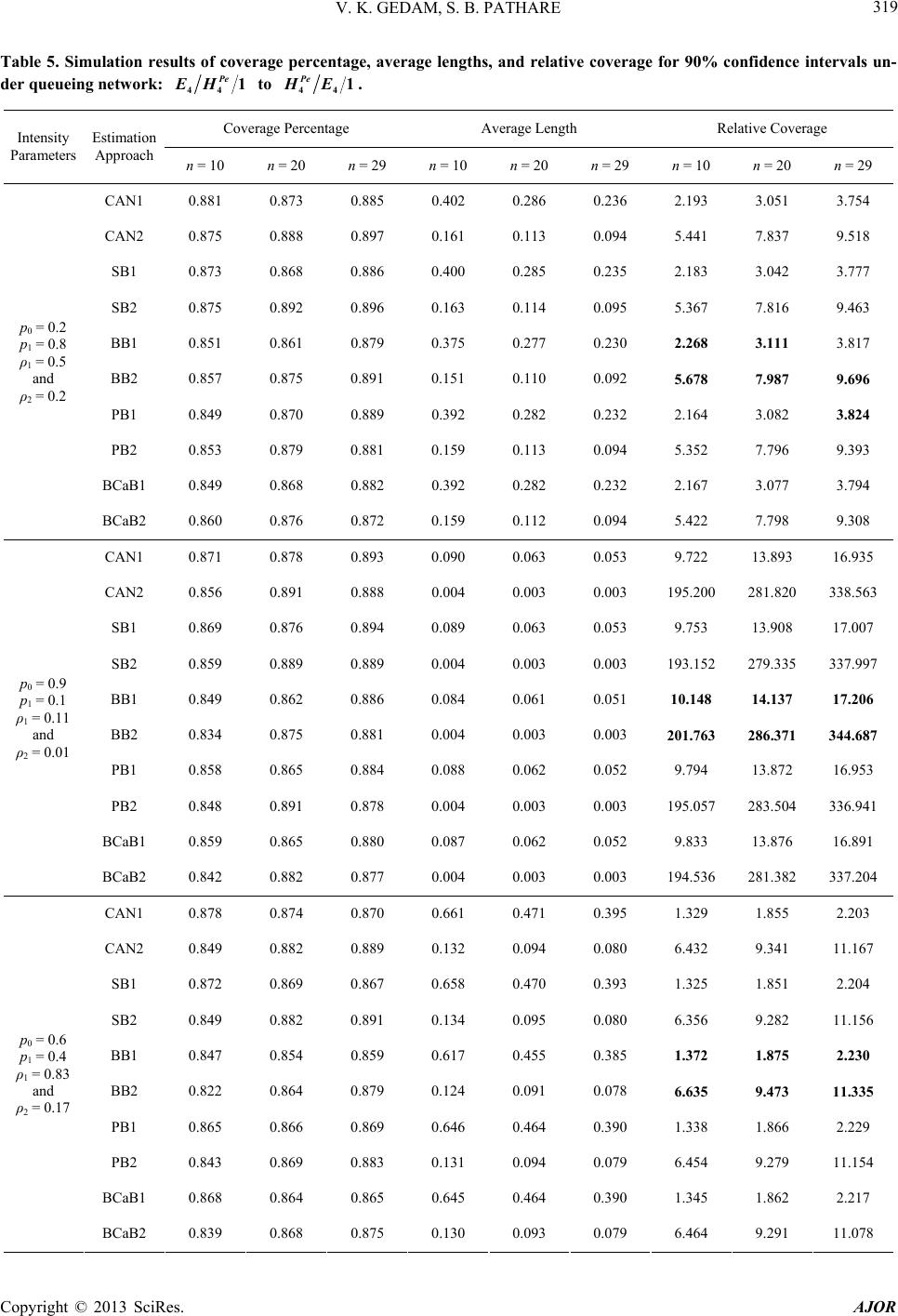

V. K. GEDAM, S. B. PATHARE
319
Table 5. Simulation results of coverage percentage, average lengths, and relative coverage for 90% confidence intervals un-
der queueing network: 44 1
Pe
EH to 44 1
Pe
HE.
Coverage Percentage Average Length Relative Coverage
Intensity
Parameters Estimation Approach n = 10 n = 20 n = 29 n = 10 n = 20 n = 29 n = 10 n = 20 n = 29
CAN1 0.881 0.873 0.885 0.402 0.286 0.236 2.193 3.051 3.754
CAN2 0.875 0.888 0.897 0.161 0.113 0.094 5.441 7.837 9.518
SB1 0.873 0.868 0.886 0.400 0.285 0.235 2.183 3.042 3.777
SB2 0.875 0.892 0.896 0.163 0.114 0.095 5.367 7.816 9.463
BB1 0.851 0.861 0.879 0.375 0.277 0.230 2.268 3.111 3.817
BB2 0.857 0.875 0.891 0.151 0.110 0.092 5.678 7.987 9.696
PB1 0.849 0.870 0.889 0.392 0.282 0.232 2.164 3.082 3.824
PB2 0.853 0.879 0.881 0.159 0.113 0.094 5.352 7.796 9.393
BCaB1 0.849 0.868 0.882 0.392 0.282 0.232 2.167 3.077 3.794
p0 = 0.2
p1 = 0.8
ρ1 = 0.5
and
ρ2 = 0.2
BCaB2 0.860 0.876 0.872 0.159 0.112 0.094 5.422 7.798 9.308
CAN1 0.871 0.878 0.893 0.090 0.063 0.053 9.722 13.893 16.935
CAN2 0.856 0.891 0.888 0.004 0.003 0.003 195.200 281.820 338.563
SB1 0.869 0.876 0.894 0.089 0.063 0.053 9.753 13.908 17.007
SB2 0.859 0.889 0.889 0.004 0.003 0.003 193.152 279.335 337.997
BB1 0.849 0.862 0.886 0.084 0.061 0.051
10.148 14.137 17.206
BB2 0.834 0.875 0.881 0.004 0.003 0.003
201.763 286.371 344.687
PB1 0.858 0.865 0.884 0.088 0.062 0.052 9.794 13.872 16.953
PB2 0.848 0.891 0.878 0.004 0.003 0.003 195.057 283.504 336.941
BCaB1 0.859 0.865 0.880 0.087 0.062 0.052 9.833 13.876 16.891
p0 = 0.9
p1 = 0.1
ρ1 = 0.11
and
ρ2 = 0.01
BCaB2 0.842 0.882 0.877 0.004 0.003 0.003 194.536 281.382 337.204
CAN1 0.878 0.874 0.870 0.661 0.471 0.395 1.329 1.855 2.203
CAN2 0.849 0.882 0.889 0.132 0.094 0.080 6.432 9.341 11.167
SB1 0.872 0.869 0.867 0.658 0.470 0.393 1.325 1.851 2.204
SB2 0.849 0.882 0.891 0.134 0.095 0.080 6.356 9.282 11.156
BB1 0.847 0.854 0.859 0.617 0.455 0.385 1.372 1.875 2.230
BB2 0.822 0.864 0.879 0.124 0.091 0.078 6.635 9.473 11.335
PB1 0.865 0.866 0.869 0.646 0.464 0.390 1.338 1.866 2.229
PB2 0.843 0.869 0.883 0.131 0.094 0.079 6.454 9.279 11.154
BCaB1 0.868 0.864 0.865 0.645 0.464 0.390 1.345 1.862 2.217
p0 = 0.6
p1 = 0.4
ρ1 = 0.83
and
ρ2 = 0.17
BCaB2 0.839 0.868 0.875 0.130 0.093 0.079 6.464 9.291 11.078

V. K. GEDAM, S. B. PATHARE
320
Continued
CAN1 0.858 0.875 0.891 0.452 0.320 0.263 1.897 2.730 3.390
CAN2 0.870 0.884 0.891 0.022 0.016 0.013 39.305 55.479 67.767
SB1 0.858 0.874 0.890 0.450 0.320 0.262 1.906 2.731 3.397
SB2 0.870 0.882 0.896 0.022 0.016 0.013 38.755 54.933 67.862
BB1 0.836 0.863 0.881 0.422 0.309 0.256 1.983 2.790 3.441
BB2 0.836 0.879 0.881 0.021 0.015 0.013
40.177 57.074 68.727
PB1 0.847 0.876 0.895 0.441 0.317 0.260 1.919 2.767 3.445
PB2 0.847 0.878 0.887 0.022 0.016 0.013 38.630 55.413 67.828
BCaB1 0.847 0.873 0.890 0.441 0.317 0.260 1.919 2.757 3.429
p0 = 0.9
p1 = 0.1
ρ1 = 0.56
and
ρ2 = 0.03
BCaB2 0.843 0.878 0.883 0.022 0.016 0.013 38.676 55.614 67.700
CAN1 0.853 0.882 0.886 0.396 0.282 0.237 2.156 3.127 3.738
CAN2 0.879 0.895 0.877 0.723 0.504 0.425 1.216 1.777 2.064
SB1 0.852 0.880 0.889 0.393 0.281 0.236 2.167 3.129 3.761
SB2 0.882 0.897 0.875 0.736 0.506 0.426 1.199 1.771 2.055
BB1 0.829 0.866 0.877 0.369 0.272 0.231 2.247 3.184 3.795
BB2 0.863 0.885 0.868 0.681 0.486 0.414 1.268 1.822 2.095
PB1 0.850 0.869 0.887 0.386 0.278 0.234 2.203 3.124 3.785
PB2 0.869 0.901 0.857 0.718 0.501 0.421 1.211 1.799 2.033
BCaB1 0.843 0.869 0.883 0.384 0.278 0.234 2.194 3.126 3.767
p0 = 0.1
p1 = 0.9
ρ1 = 0.5
and
ρ2 = 0.9
BCaB2 0.869 0.898 0.859 0.713 0.499 0.421 1.219 1.799 2.043
CAN1 0.858 0.890 0.891 0.503 0.358 0.295 1.707 2.485 3.018
CAN2 0.871 0.857 0.891 0.595 0.427 0.354 1.463 2.005 2.517
SB1 0.852 0.892 0.888 0.500 0.357 0.294 1.704 2.497 3.018
SB2 0.875 0.858 0.897 0.605 0.430 0.355 1.447 1.995 2.525
BB1 0.825 0.880 0.883 0.469 0.346 0.288 1.759 2.546 3.066
BB2 0.849 0.845 0.883 0.559 0.412 0.345 1.517 2.051 2.559
PB1 0.832 0.878 0.891 0.491 0.353 0.291 1.693 2.487 3.057
PB2 0.848 0.854 0.884 0.591 0.425 0.352 1.436 2.010 2.514
BCaB1 0.823 0.873 0.883 0.491 0.353 0.291 1.678 2.472 3.031
p0 = 0.4
p1 = 0.6
ρ1 = 0.63
and
ρ2 = 0.75
BCaB2 0.853 0.848 0.881 0.586 0.424 0.351 1.455 2.001 2.510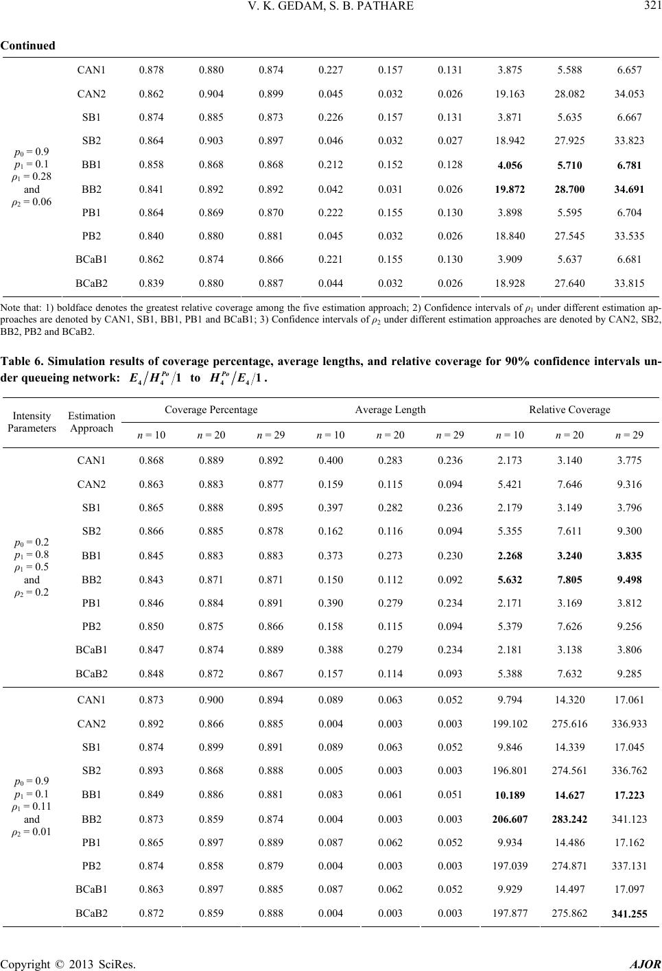

V. K. GEDAM, S. B. PATHARE
321
Continued
CAN1 0.878 0.880 0.874 0.227 0.157 0.131 3.875 5.588 6.657
CAN2 0.862 0.904 0.899 0.045 0.032 0.026 19.163 28.082 34.053
SB1 0.874 0.885 0.873 0.226 0.157 0.131 3.871 5.635 6.667
SB2 0.864 0.903 0.897 0.046 0.032 0.027 18.942 27.925 33.823
BB1 0.858 0.868 0.868 0.212 0.152 0.128 4.056 5.710 6.781
BB2 0.841 0.892 0.892 0.042 0.031 0.026 19.872 28.700 34.691
PB1 0.864 0.869 0.870 0.222 0.155 0.130 3.898 5.595 6.704
PB2 0.840 0.880 0.881 0.045 0.032 0.026 18.840 27.545 33.535
BCaB1 0.862 0.874 0.866 0.221 0.155 0.130 3.909 5.637 6.681
p0 = 0.9
p1 = 0.1
ρ1 = 0.28
and
ρ2 = 0.06
BCaB2 0.839 0.880 0.887 0.044 0.032 0.026 18.928 27.640 33.815
Note that: 1) boldface denotes the greatest relative coverage among the five estimation approach; 2) Confidence intervals of ρ1 under different estimation ap-
proaches are denoted by CAN1, SB1, BB1, PB1 and BCaB1; 3) Confidence intervals of ρ2 under different estimation approaches are denoted by CAN2, SB2,
BB2, PB2 and BCaB2.
Table 6. Simulation results of coverage percentage, average lengths, and relative coverage for 90% confidence intervals un-
der queueing network: 44 1
Po
EH to 44 1
Po
HE.
Coverage Percentage Average Length Relative Coverage
Intensity
Parameters Estimation Approach n = 10 n = 20 n = 29 n = 10 n = 20 n = 29 n = 10 n = 20 n = 29
CAN1 0.868 0.889 0.892 0.400 0.283 0.236 2.173 3.140 3.775
CAN2 0.863 0.883 0.877 0.159 0.115 0.094 5.421 7.646 9.316
SB1 0.865 0.888 0.895 0.397 0.282 0.236 2.179 3.149 3.796
SB2 0.866 0.885 0.878 0.162 0.116 0.094 5.355 7.611 9.300
BB1 0.845 0.883 0.883 0.373 0.273 0.230 2.268 3.240 3.835
BB2 0.843 0.871 0.871 0.150 0.112 0.092 5.632 7.805 9.498
PB1 0.846 0.884 0.891 0.390 0.279 0.234 2.171 3.169 3.812
PB2 0.850 0.875 0.866 0.158 0.115 0.094 5.379 7.626 9.256
BCaB1 0.847 0.874 0.889 0.388 0.279 0.234 2.181 3.138 3.806
p0 = 0.2
p1 = 0.8
ρ1 = 0.5
and
ρ2 = 0.2
BCaB2 0.848 0.872 0.867 0.157 0.114 0.093 5.388 7.632 9.285
CAN1 0.873 0.900 0.894 0.089 0.063 0.052 9.794 14.320 17.061
CAN2 0.892 0.866 0.885 0.004 0.003 0.003 199.102 275.616 336.933
SB1 0.874 0.899 0.891 0.089 0.063 0.052 9.846 14.339 17.045
SB2 0.893 0.868 0.888 0.005 0.003 0.003 196.801 274.561 336.762
BB1 0.849 0.886 0.881 0.083 0.061 0.051
10.189 14.627 17.223
BB2 0.873 0.859 0.874 0.004 0.003 0.003 206.607 283.242 341.123
PB1 0.865 0.897 0.889 0.087 0.062 0.052 9.934 14.486 17.162
PB2 0.874 0.858 0.879 0.004 0.003 0.003 197.039 274.871 337.131
BCaB1 0.863 0.897 0.885 0.087 0.062 0.052 9.929 14.497 17.097
p0 = 0.9
p1 = 0.1
ρ1 = 0.11
and
ρ2 = 0.01
BCaB2 0.872 0.859 0.888 0.004 0.003 0.003 197.877 275.862 341.255

V. K. GEDAM, S. B. PATHARE
322
Continued
CAN1 0.870 0.888 0.870 0.661 0.473 0.391 1.316 1.878 2.226
CAN2 0.852 0.890 0.894 0.134 0.095 0.080 6.378 9.414 11.213
SB1 0.867 0.884 0.871 0.658 0.471 0.390 1.318 1.875 2.236
SB2 0.859 0.891 0.893 0.135 0.095 0.080 6.347 9.388 11.170
BB1 0.851 0.872 0.864 0.618 0.456 0.381 1.378 1.912 2.267
BB2 0.835 0.875 0.887 0.126 0.091 0.078 6.651 9.588 11.401
PB1 0.863 0.886 0.868 0.646 0.466 0.386 1.336 1.901 2.247
PB2 0.843 0.872 0.888 0.132 0.094 0.079 6.369 9.293 11.214
BCaB1 0.862 0.885 0.863 0.645 0.466 0.386 1.336 1.900 2.236
p0 = 0.6
p1 = 0.4
ρ1 = 0.83
and
ρ2 = 0.17
BCaB2 0.837 0.870 0.885 0.132 0.094 0.079 6.362 9.302 11.196
CAN1 0.868 0.892 0.881 0.451 0.313 0.260 1.924 2.848 3.389
CAN2 0.855 0.889 0.888 0.022 0.016 0.013 38.912 56.159 67.891
SB1 0.868 0.890 0.882 0.449 0.312 0.259 1.932 2.850 3.400
SB2 0.855 0.886 0.889 0.022 0.016 0.013 38.389 55.660 67.803
BB1 0.846 0.873 0.872 0.421 0.303 0.254 2.009 2.885 3.438
BB2 0.837 0.871 0.881 0.021 0.015 0.013
40.525 56.991 69.056
PB1 0.852 0.885 0.871 0.441 0.309 0.257 1.931 2.868 3.388
PB2 0.841 0.891 0.884 0.022 0.016 0.013 38.677 56.728 68.080
BCaB1 0.853 0.878 0.872 0.440 0.308 0.257 1.940 2.846 3.390
p0 = 0.9
p1 = 0.1
ρ1 = 0.56
and
ρ2 = 0.03
BCaB2 0.839 0.892 0.886 0.022 0.016 0.013 38.827 56.980 68.421
CAN1 0.856 0.889 0.896 0.393 0.283 0.239 2.178 3.137 3.754
CAN2 0.866 0.895 0.888 0.727 0.508 0.427 1.191 1.763 2.081
SB1 0.851 0.891 0.896 0.391 0.283 0.238 2.174 3.152 3.759
SB2 0.862 0.889 0.889 0.738 0.510 0.428 1.168 1.742 2.077
BB1 0.829 0.878 0.886 0.367 0.274 0.232 2.259 3.206 3.816
BB2 0.838 0.882 0.882 0.684 0.490 0.416 1.225 1.798 2.121
PB1 0.851 0.888 0.882 0.385 0.279 0.236 2.213 3.179 3.731
PB2 0.836 0.876 0.874 0.722 0.504 0.424 1.158 1.739 2.064
BCaB1 0.848 0.881 0.885 0.384 0.279 0.236 2.210 3.155 3.746
p0 = 0.1
p1 = 0.9
ρ1 = 0.5
and
ρ2 = 0.9
BCaB2 0.840 0.875 0.880 0.716 0.502 0.423 1.173 1.742 2.083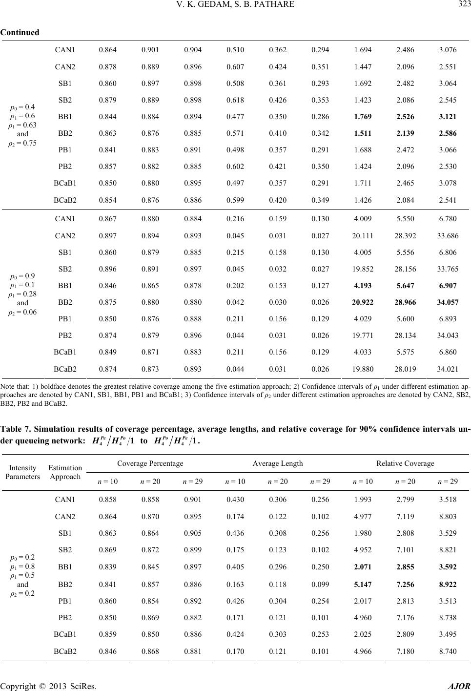

V. K. GEDAM, S. B. PATHARE
323
Continued
CAN1 0.864 0.901 0.904 0.510 0.362 0.294 1.694 2.486 3.076
CAN2 0.878 0.889 0.896 0.607 0.424 0.351 1.447 2.096 2.551
SB1 0.860 0.897 0.898 0.508 0.361 0.293 1.692 2.482 3.064
SB2 0.879 0.889 0.898 0.618 0.426 0.353 1.423 2.086 2.545
BB1 0.844 0.884 0.894 0.477 0.350 0.286 1.769 2.526 3.121
BB2 0.863 0.876 0.885 0.571 0.410 0.342 1.511 2.139 2.586
PB1 0.841 0.883 0.891 0.498 0.357 0.291 1.688 2.472 3.066
PB2 0.857 0.882 0.885 0.602 0.421 0.350 1.424 2.096 2.530
BCaB1 0.850 0.880 0.895 0.497 0.357 0.291 1.711 2.465 3.078
p0 = 0.4
p1 = 0.6
ρ1 = 0.63
and
ρ2 = 0.75
BCaB2 0.854 0.876 0.886 0.599 0.420 0.349 1.426 2.084 2.541
CAN1 0.867 0.880 0.884 0.216 0.159 0.130 4.009 5.550 6.780
CAN2 0.897 0.894 0.893 0.045 0.031 0.027 20.111 28.392 33.686
SB1 0.860 0.879 0.885 0.215 0.158 0.130 4.005 5.556 6.806
SB2 0.896 0.891 0.897 0.045 0.032 0.027 19.852 28.156 33.765
BB1 0.846 0.865 0.878 0.202 0.153 0.127 4.193 5.647 6.907
BB2 0.875 0.880 0.880 0.042 0.030 0.026
20.922 28.966 34.057
PB1 0.850 0.876 0.888 0.211 0.156 0.129 4.029 5.600 6.893
PB2 0.874 0.879 0.896 0.044 0.031 0.026 19.771 28.134 34.043
BCaB1 0.849 0.871 0.883 0.211 0.156 0.129 4.033 5.575 6.860
p0 = 0.9
p1 = 0.1
ρ1 = 0.28
and
ρ2 = 0.06
BCaB2 0.874 0.873 0.893 0.044 0.031 0.026 19.880 28.019 34.021
Note that: 1) boldface denotes the greatest relative coverage among the five estimation approach; 2) Confidence intervals of ρ1 under different estimation ap-
proaches are denoted by CAN1, SB1, BB1, PB1 and BCaB1; 3) Confidence intervals of ρ2 under different estimation approaches are denoted by CAN2, SB2,
BB2, PB2 and BCaB2.
Table 7. Simulation results of coverage percentage, average lengths, and relative coverage for 90% confidence intervals un-
der queueing network: 44 1
Pe Po
HH to 44 1
Po Pe
HH .
Coverage Percentage Average Length Relative Coverage
Intensity
Parameters Estimation Approach n = 10 n = 20 n = 29 n = 10 n = 20 n = 29 n = 10 n = 20 n = 29
CAN1 0.858 0.858 0.901 0.430 0.306 0.256 1.993 2.799 3.518
CAN2 0.864 0.870 0.895 0.174 0.122 0.102 4.977 7.119 8.803
SB1 0.863 0.864 0.905 0.436 0.308 0.256 1.980 2.808 3.529
SB2 0.869 0.872 0.899 0.175 0.123 0.102 4.952 7.101 8.821
BB1 0.839 0.845 0.897 0.405 0.296 0.250 2.071 2.855 3.592
BB2 0.841 0.857 0.886 0.163 0.118 0.099 5.147 7.256 8.922
PB1 0.860 0.854 0.892 0.426 0.304 0.254 2.017 2.813 3.513
PB2 0.850 0.869 0.882 0.171 0.121 0.101 4.960 7.176 8.738
BCaB1 0.859 0.850 0.886 0.424 0.303 0.253 2.025 2.809 3.495
p0 = 0.2
p1 = 0.8
ρ1 = 0.5
and
ρ2 = 0.2
BCaB2 0.846 0.868 0.881 0.170 0.121 0.101 4.966 7.180 8.740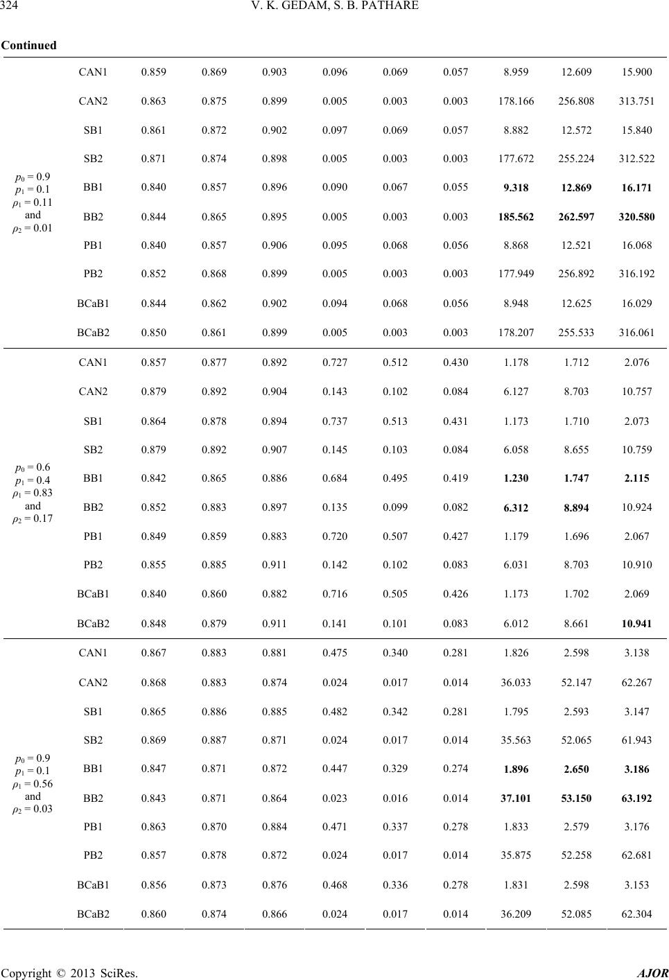

V. K. GEDAM, S. B. PATHARE
324
Continued
CAN1 0.859 0.869 0.903 0.096 0.069 0.057 8.959 12.609 15.900
CAN2 0.863 0.875 0.899 0.005 0.003 0.003 178.166 256.808 313.751
SB1 0.861 0.872 0.902 0.097 0.069 0.057 8.882 12.572 15.840
SB2 0.871 0.874 0.898 0.005 0.003 0.003 177.672 255.224 312.522
BB1 0.840 0.857 0.896 0.090 0.067 0.055 9.318 12.869 16.171
BB2 0.844 0.865 0.895 0.005 0.003 0.003
185.562 262.597 320.580
PB1 0.840 0.857 0.906 0.095 0.068 0.056 8.868 12.521 16.068
PB2 0.852 0.868 0.899 0.005 0.003 0.003 177.949 256.892 316.192
BCaB1 0.844 0.862 0.902 0.094 0.068 0.056 8.948 12.625 16.029
p0 = 0.9
p1 = 0.1
ρ1 = 0.11
and
ρ2 = 0.01
BCaB2 0.850 0.861 0.899 0.005 0.003 0.003 178.207 255.533 316.061
CAN1 0.857 0.877 0.892 0.727 0.512 0.430 1.178 1.712 2.076
CAN2 0.879 0.892 0.904 0.143 0.102 0.084 6.127 8.703 10.757
SB1 0.864 0.878 0.894 0.737 0.513 0.431 1.173 1.710 2.073
SB2 0.879 0.892 0.907 0.145 0.103 0.084 6.058 8.655 10.759
BB1 0.842 0.865 0.886 0.684 0.495 0.419 1.230 1.747 2.115
BB2 0.852 0.883 0.897 0.135 0.099 0.082 6.312 8.894 10.924
PB1 0.849 0.859 0.883 0.720 0.507 0.427 1.179 1.696 2.067
PB2 0.855 0.885 0.911 0.142 0.102 0.083 6.031 8.703 10.910
BCaB1 0.840 0.860 0.882 0.716 0.505 0.426 1.173 1.702 2.069
p0 = 0.6
p1 = 0.4
ρ1 = 0.83
and
ρ2 = 0.17
BCaB2 0.848 0.879 0.911 0.141 0.101 0.083 6.012 8.661
10.941
CAN1 0.867 0.883 0.881 0.475 0.340 0.281 1.826 2.598 3.138
CAN2 0.868 0.883 0.874 0.024 0.017 0.014 36.033 52.147 62.267
SB1 0.865 0.886 0.885 0.482 0.342 0.281 1.795 2.593 3.147
SB2 0.869 0.887 0.871 0.024 0.017 0.014 35.563 52.065 61.943
BB1 0.847 0.871 0.872 0.447 0.329 0.274 1.896 2.650 3.186
BB2 0.843 0.871 0.864 0.023 0.016 0.014 37.101 53.150 63.192
PB1 0.863 0.870 0.884 0.471 0.337 0.278 1.833 2.579 3.176
PB2 0.857 0.878 0.872 0.024 0.017 0.014 35.875 52.258 62.681
BCaB1 0.856 0.873 0.876 0.468 0.336 0.278 1.831 2.598 3.153
p0 = 0.9
p1 = 0.1
ρ1 = 0.56
and
ρ2 = 0.03
BCaB2 0.860 0.874 0.866 0.024 0.017 0.014 36.209 52.085 62.304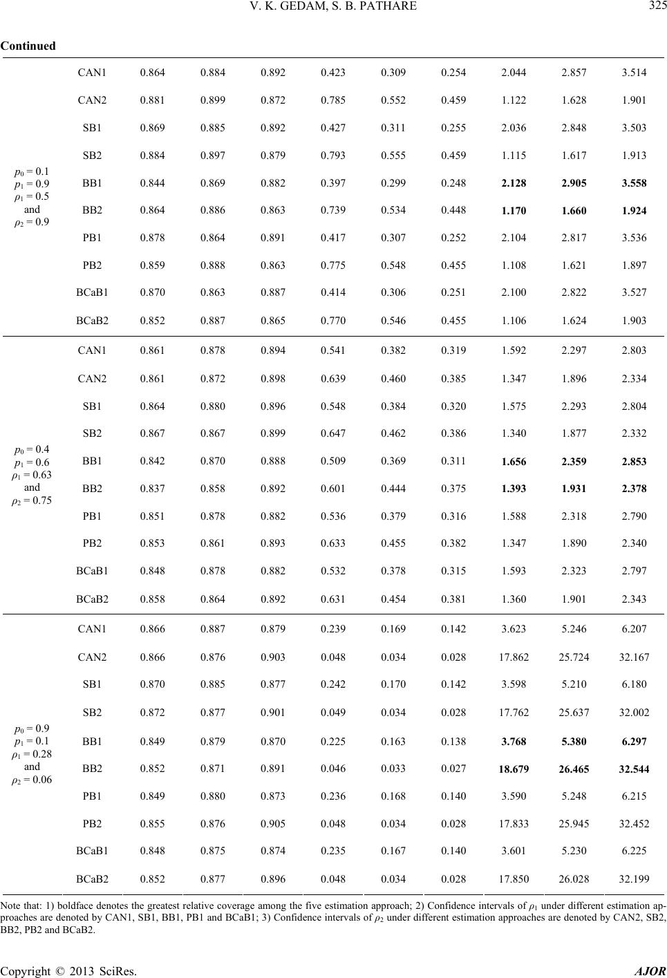

V. K. GEDAM, S. B. PATHARE
325
Continued
CAN1 0.864 0.884 0.892 0.423 0.309 0.254 2.044 2.857 3.514
CAN2 0.881 0.899 0.872 0.785 0.552 0.459 1.122 1.628 1.901
SB1 0.869 0.885 0.892 0.427 0.311 0.255 2.036 2.848 3.503
SB2 0.884 0.897 0.879 0.793 0.555 0.459 1.115 1.617 1.913
BB1 0.844 0.869 0.882 0.397 0.299 0.248 2.128 2.905 3.558
BB2 0.864 0.886 0.863 0.739 0.534 0.448 1.170 1.660 1.924
PB1 0.878 0.864 0.891 0.417 0.307 0.252 2.104 2.817 3.536
PB2 0.859 0.888 0.863 0.775 0.548 0.455 1.108 1.621 1.897
BCaB1 0.870 0.863 0.887 0.414 0.306 0.251 2.100 2.822 3.527
p0 = 0.1
p1 = 0.9
ρ1 = 0.5
and
ρ2 = 0.9
BCaB2 0.852 0.887 0.865 0.770 0.546 0.455 1.106 1.624 1.903
CAN1 0.861 0.878 0.894 0.541 0.382 0.319 1.592 2.297 2.803
CAN2 0.861 0.872 0.898 0.639 0.460 0.385 1.347 1.896 2.334
SB1 0.864 0.880 0.896 0.548 0.384 0.320 1.575 2.293 2.804
SB2 0.867 0.867 0.899 0.647 0.462 0.386 1.340 1.877 2.332
BB1 0.842 0.870 0.888 0.509 0.369 0.311 1.656 2.359 2.853
BB2 0.837 0.858 0.892 0.601 0.444 0.375 1.393 1.931 2.378
PB1 0.851 0.878 0.882 0.536 0.379 0.316 1.588 2.318 2.790
PB2 0.853 0.861 0.893 0.633 0.455 0.382 1.347 1.890 2.340
BCaB1 0.848 0.878 0.882 0.532 0.378 0.315 1.593 2.323 2.797
p0 = 0.4
p1 = 0.6
ρ1 = 0.63
and
ρ2 = 0.75
BCaB2 0.858 0.864 0.892 0.631 0.454 0.381 1.360 1.901 2.343
CAN1 0.866 0.887 0.879 0.239 0.169 0.142 3.623 5.246 6.207
CAN2 0.866 0.876 0.903 0.048 0.034 0.028 17.862 25.724 32.167
SB1 0.870 0.885 0.877 0.242 0.170 0.142 3.598 5.210 6.180
SB2 0.872 0.877 0.901 0.049 0.034 0.028 17.762 25.637 32.002
BB1 0.849 0.879 0.870 0.225 0.163 0.138 3.768 5.380 6.297
BB2 0.852 0.871 0.891 0.046 0.033 0.027
18.679 26.465 32.544
PB1 0.849 0.880 0.873 0.236 0.168 0.140 3.590 5.248 6.215
PB2 0.855 0.876 0.905 0.048 0.034 0.028 17.833 25.945 32.452
BCaB1 0.848 0.875 0.874 0.235 0.167 0.140 3.601 5.230 6.225
p0 = 0.9
p1 = 0.1
ρ1 = 0.28
and
ρ2 = 0.06
BCaB2 0.852 0.877 0.896 0.048 0.034 0.028 17.850 26.028 32.199
Note that: 1) boldface denotes the greatest relative coverage among the five estimation approach; 2) Confidence intervals of ρ1 under different estimation ap-
proaches are denoted by CAN1, SB1, BB1, PB1 and BCaB1; 3) Confidence intervals of ρ2 under different estimation approaches are denoted by CAN2, SB2,
BB2, PB2 and BCaB2.

V. K. GEDAM, S. B. PATHARE
326
are decreasing as p0 approaches 1 (p1 approaches 0) but
both coverage percentages and relative coverage are in-
creasing as p0 approaches 1 (p1 approaches 0).
Also we find that average lengths are decreasing with
sample size n but both coverage percentages and relative
coverage are increasing with sample size n. From Tables
3 to 7 one can observe that the coverage percentage can
approach to 90% when n increases up to 29.
1) In queueing network models 41ME to 41EM
and 41
Pe
MH to 41
Pe
H
M, the estimation approach
CAN and BB has the greatest relative coverage among
the five confidence intervals for 1

and 2

respectively
for diffe r ent values of p0 and p1.
2) In queueing network models 44
1
Pe
EH to
44
1
Pe
H
E, 44 1
Po
EH to 44 1
Po
H
E and 44 1
Pe Po
HH
to 44 1
Po Pe
HH , the estimation approach BB has the
greatest relative coverage among the five confidence
intervals for 1

and 2

for different values of p0 and p1.
3) Average lengths are decreasing as sample size n in-
creases for both 1

and 2

. Also relative coverage in-
creases with n for 1

and 2

.
4) Some poor coverage percentage of above confi-
dence intervals with respect to the nominal level 90%
may be due to small sample size n.
8. Conclusion
This paper provides the interval esti mations of intens ities
1

and 2

for an open qu eueing network w ith feedb ack.
Different estimation approaches CAN, SB, BB, PB and
BCaB are applied to produce confidence intervals for
intensities 1

and 2

. The relative coverage is adopted
to understand, compare and assess performance of the
resulted confidence intervals. From simulation study it is
clear that CAN and BB method has the best performance
on interval estimation of intensities 1

and 2

for
1
M
G to 1
M
G queueing network and BB method
has the best performance on interval estimation of inten-
sities 1

and 2

for 1GG to 1GG queueing net-
work with short run data. And ap proach is easily applied
to practical queueing network system such as all types of
open, closed, mixed queueing networks as well as cyclic,
retrial queueing models.
REFERENCES
[1] R. L. Disney, “Random Flow in Queueing Networks: A
Review and a Critique,” A.I.E.E. Transactions, Vo l. 8, No.
1, 1975, pp. 268-288.
[2] P. J. Burke, “Proof of Conjecture on the Inter-Arrival
Time Distribution in M/M/1 Queue with Feedback,”
IEEE Transactions on Communications, Vol. 24, No. 5,
1976, pp. 175-178. doi:10.1109/TCOM.1976.1093335
[3] F.J. Beautler and B. Melamed, “Decomposition and Cus-
tomer Streams of Feedback Networks of Queues in Equi-
librium,” Operation Research, Vol. 26, No. 6, 1978, pp.
1059-1072. doi:10.1287/opre.26.6.1059
[4] J. R. Jackson, “Networks of Waiting Lines,” Operations
Research, Vol. 5, No. 4, 1957, pp. 518-521.
doi:10.1287/opre.5.4.518
[5] B. Simon and R. D. Foley, “Some Results on Sojourn
Times in Acyclic Jackson Network,” Management Sci-
ence, Vol. 25, No. 10, 1979, pp. 1027-1034.
doi:10.1287/mnsc.25.10.1027
[6] B. Melamed, “Sojourn Times in Queueing Networks,”
Technical Report, Department of Industrial Engineering
and Manage ment Sciences, Nort hwestern Univer sity, Evan-
ston, 1980.
[7] R. L. Disney and P. C. Kiessler, “Traffic Processes in
Queueing Networks: A Markov Renewal Approach,”
Johns Hopkins University Press, Baltimore, 1987.
[8] D. Thiruvaiyaru, I. V. Basava and U. N. Bhat, “Estima-
tion for a Class of Simple Queueing Network,” Queueing
Systems, Vol. 9, No. 3, 1991, pp. 301-312.
doi:10.1007/BF01158468
[9] D. Thiruvaiyaru and I. V. Basava, “Maximum Likelihood
Estimation for Queueing Networks,” In: B. L. S. Prakasa
Rao and B. R. Bhat, Eds., Stochastic Processes and Sta-
tistical Inference, New Age International Publications,
New Delhi, 1996, pp. 132-149.
[10] L. Kleinrock, “Queueing Systems, Vol. II: Computer Ap-
plications,” John Wiley & Sons, New York, 1976.
[11] P. J. Denning and J. P. Buzen, “The Operational Analysis
of Queueing Network Models,” ACM Computing Surveys,
Vol. 10, No. 3, 1978, pp. 225-261.
[12] B. Efron, “Bootstrap Methods: Another Look at the Jack-
knife,” Annals of Statistics, Vol. 7, No. 1, 1979, pp. 1-26.
doi:10.1214/aos/1176344552
[13] B. Efron, “The Jackknife, the Bootstrap, and Other Re-
sampling Plans,” CBMS-NSF Regional Conference Series
in Applied Mathematics, Monograph 38, SIAM, Phila-
delphia, 1982.
[14] B. Efron, “Better Bootstrap Confidence Intervals,” Jour-
nal of the American Statistical Association, Vol. 82, No.
397, 1987, pp. 171-200. doi:10.2307/2289144
[15] D. B. Rubin, “The Bayesian Bootstrap,” The Annals of
Statistics, Vol. 9, No. 1, 1981, pp. 130-134.
doi:10.1214/aos/1176345338
[16] R. G. Miller, “The Jackknife: A Review,” Biometrika,
Vol. 61, No. 1, 1974, pp. 1-15.
[17] Y.-K. Chu and J.-C. Ke, “Confidence Intervals of Mean
Response Time for an M/G/1 Queueing System: Boot-
strap Simulation,” Applied Mathematics and Computation,
Vol. 180, No. 1, 2006, pp. 255-263.
doi:10.1016/j.amc.2005.11.145
[18] Y. K. Chu and J.C. Ke, Interval Estimation of Mean Re-
sponse Time for a G/M/1 Queueing System: Empirical
Laplace Function Approach,” Mathematical Methods in
the Applied Sciences, Vol. 30, No. 6, 2006, pp. 707-715.
doi:10.1002/mma.806
[19] J. C. Ke and Y. K. Chu, “Nonparametric and Simulated
Analysis of Intensity for Queueing System,” Applied

V. K. GEDAM, S. B. PATHARE
327
Mathematics and Computation, Vol. 183, No. 2, 2006, pp.
1280-1291. doi:10.1016/j.amc.2006.05.163
[20] J. C. Ke and Y. K. Chu, “Comparison on Five Estimation
Approaches of Intensity for a Queueing Sy stem with Short
Run,” Computational Statistics, Vol. 24, No. 4, 2009, pp.
567-582.
[21] R. V. Hogg, A. T. Craig and J. W. McKean, “Introduction
to Mathematical Statistics,” 6th Edition, Prentice-Hall,
Inc., Upper Saddle River, 2011.