 American Journal of Operations Research, 2013, 3, 289-298 http://dx.doi.org/10.4236/ajor.2013.32026 Published Online March 2013 (http://www.scirp.org/journal/ajor) Generating Efficient Solutions in Bilevel Multi-Objective Programming Problems Calice Olivier Pieume1, Patrice Marcotte2, Laure Pauline Fotso3, Patrick Siarry4 1Department of Mathematics, Faculty of Science, University of Yaoundé I, Yaoundé, Cameroon 2Department of Computer Science and Operations Research, University of Montreal, Montreal, Canada 3Department of Computer Sciences, Faculty of Science, University of Yaoundé I, Yaoundé, Cameroon 4LISSI, Faculty of Sciences and Technology, University of Paris XII Val-de-Marne, Créteil, France Email: olivier.pieume@poledakar.org, marcotte@iro.umontreal.ca, laurepfotso@ballstate.bsu.edu, siarry@univ-paris12.fr Received January 2, 2013; revised February 8, 2013; accepted February 17, 2013 ABSTRACT In this paper, we address bilevel multi-objective programming problems (BMPP) in which the decision maker at each level has multiple objective functions conflicting with each other. Given a BMPP, we show how to construct two artifi- cial multiobjective programming problems such that any point that is efficient for both the two problems is an efficient solution of the BMPP. Some necessary and sufficient conditions for which the obtained result is applicable are provided. A complete procedure of the implementation of an algorithm for generating efficient solutions for the linear case of BMPP is presented. A numerical example is provided to illustrate how the algorithm operates. Keywords: Multi-Objective Programming; Bilevel Programming; Efficient Solution; Efficient Edge; Hierarchical Systems 1. Introduction Bilevel programming is proposed in the literature for dealing with hierarchical systems. It involves two opti- mization problems where the data of the first one is im- plicitly determined by the solution of the second. Each decision maker (DM) tries to optimize its own objective function without considering the objective of the other party, but the decision of each party affects the objective value of the one party as well as the decision space. Bilevel problems occur in diverse applications, such as transportation, economics, ecology, engineering and oth- ers. Standard bilevel programming problems where each DM has only one objective have been extensively studied in the literature [1,2]. Recent books by Dempe [3] and J. F. Bard [4] present results, applications and solution methods for standard formulation where the objective functions and constraints are not necessarily linear. However, despite their multiple applications [5], the spe- cial case of bilevel programming problems where each DM has more than one objective function has not yet received a broad attention in the literature. We have found only about a dozen articles related to this class of problems in the literature [6-11]. The lack of work is due certainly to the difficulty of searching and defining opti- mal solutions. Contrarily to the standard two levels pro- gramming problem where it is usually assumed that the set of rational responses of the follower is a singleton, in the bilevel multi-objective problem, the lower level op- timization problem has a number of trade-off optimal solutions and the task of the upper level is to focus its search on multiple trade-off solutions which are members of optimal trade-off solutions of lower level optimization problem. Bilevel Multi-objective Programming Problem is then computationally more complex than the conven- tional Multi-Objective Programming Problem or a bilevel Programming Problem. In this paper, we address bilevel multi-objective prob- lems in which the decision maker at each level has mul- tiple objective functions conflicting with each other. Given a BMPP, we show how to construct two artificial multi-objective programming problems such that any point that is efficient for both the two problems is an ef- ficient solution of the BMPP. Based on this result, we provided a general algorithm for generating efficient so- lutions of BMPP. A complete procedure of its imple- mentation for the linear case of BMPP is presented. A numerical example is provided to illustrate how the algo- rithm operates. The paper is organized as follows. In the next section, in addition to some notations and definitions that are given, we present the formulation of the problem on C opyright © 2013 SciRes. AJOR  C. O. PIEUME ET AL. 290 which we will focus. In Section 3, we show how to con- struct two artificial multi-objective programming prob- lems whose resolutions can permit to generate efficient solutions of BMPP . Section 4 provides some necessary and sufficient conditions for the application of the ob- tained relation. Section 5, is devoted essentially to the implementation of the algorithm for the generation of efficient points in bilevel linear multi-objective pro- gramming problems. We give in Section 6 a numerical example to illustrate the proposed algorithm. Finally, the paper is concluded in Section 7. 2. The Bilevel Multi-Objective Programming Problem (BMPP) 2.1. Preliminaries and Notations A multi-objective programming problem is formulated in general as follows: “min” 12 hxh xh ,,, Q xh x . tx U :hR R R (MO P P) where nQ is the objective function vectors and the set of constraints. n In order to solve (MOPP), it is necessary to define how objective function vectors U ,,, Q xh x 12 hxh should be compared for different alternatives U . So one must define on hU Q R the order that should be used for the comparison. Due to the fact that, for , there is no canonical (total) order in as there is on R, one can just define partial orders on Q2 hU KQ R. Let K be an ar- bitrary cone such that , a binary relation with respect to the cone K (noted ≤K) can be defined by: K abaK yhU b if and only if Partial orders introduced by closed pointed convex cones are the most used. Due to the fact that it could not be possible to find a solution that optimize simultane- ously all the objective functions, a weaker concept, the concept of Non-dominated point is used. Definiti o n 1 A point 0is a Non-dominated point with re- spect to the cone K if and only if there does not exist a point hU, 0 such that 0. If 6yKyy yy is a non-dominated point with respect to the cone K, then U such that hx is called Pareto-optimal point with respect to the cone K. The following definition of efficient points is the most used in the literature [12-15]. Definitio n 2 A feasible point U is called Pareto-optimal if there does not exist U , ,,, Q Q h x h x such that 12 12 ,,hxhx hx hx and 12 12 ,,, , ,,. Q Q hxhxh x hxhxh x If is Pareto-optimal then is called Non- dominated point. hx The efficient (or Pareto optimal) solutions are then so- lutions that cannot be improved in one objective function without deteriorating their performance in at least one of the rest. Let us remark that Definition 2 is a particular case of Definition 1 where the cone used is \0Rq Q Solving a multi-objective optimization problem con- sists in finding a part or the whole set of efficient points and to present it for evaluation to the Decision maker (DM). The choice of the DM is then considered as the optimal solution of the multi-objective optimization problem. . 2.2. The Optimistic Formulation of BMPP A standard Bilevel Programming Problem (BPP) can be formulated as follows: 0 min , min,subject tosolves .,0 yY xX Gx fxy Fxy yst gxy (BPP) 12 ,, :, nn FxX RyRXYY R ,:X YR , are the outer (planner’s or leader’s) problem objective function and the inner (behavioral or follower’s) problem objective function respectively; Gg are inequality constraints. The decision variable of the leader is x and that of the inner problem is y. When the objective functions f and the con- straints ,Gg of the upper-level and lower-level prob- lems are all linear, the resulting problem is called Bilevel Linear Programming Problem (BLPP) or Linear Stack- elberg Game. If F and f are vector value functions 12 1122 :and: nn mnn m FRRR fRRR , then one speak of bilevel multi-objective programming problems (BMPP). The formulation of a bilevel multi-objective programming problem (BMPP) can be given as follows: 1 2 1 1 min,,, ,, 0 min,,,,, .solves .,0 m xX m yY FxyFxyFxy Gx fxyfxyf xy st ystgxy (BPP) Let us denote by Rx, the set of rational responses of the follower for each decision x of the leader, it is de- Copyright © 2013 SciRes. AJOR  C. O. PIEUME ET AL. 291 fined as the set of Pareto-optimal points of the following problem: 2 1 min,,, ,, m yY fxyfxyf xy ., 0stgxy 1 , , m With this notation, we have the following formulation of BMPP: 1 min,,, 0 subject to xX xyF xy Gx yRx F xy Let denote by the feasible space of BMPP defined by: and 12 ,0 nn yRRGx yRx 1 , , m The optimistic formulation of BMPP is given by: 1 , min,,, subject to, xy xyF xy xy F xy (BMPP’) The following definition holds. Definitio n 3 , y is an efficient solution of BMPP’ if and only if ,xy a nd ,xy , ,,,, xy such that 12 12 ,, ,,, ,, FxyFxy xy Fxy xy , ,,,, xy and 12 12 ,, ,,, ,, F xyFxy xy Fxy xy The main goal of this paper is to present an approach for generating efficient points of BMPP’. Throughout the rest of the paper, the set of efficient point of a multi-objective optimization problem defined by a vector value function h on a feasible set U with re- spect to a cone K will be noted: ,,EhU 1 1 \0 mm KR K. If one speaks of efficient point without making a reference to a cone, it is will be with respect to Definition 2. We con- sider also the following notations: , 1 2\0 mm KR 2 2, 1 m R YR, , 2 m 0and 12 ,/ nn xyR GxR y Rx and S denotes the whole set of efficient solutions of prob- lem BMPP’. 3. Generating Efficient Points for BMPP’ Let us consider the following multi-objective program- ming problem, constructed from the data of (BMPP’): 1 , min,,,, ., xy fxy fxy stxyZ Let 2 21 3\0 0 mmn KR and be as defined above. Theorem 1: 3 K Proof: It is a slight modified version of Theorem 4.1 given in [7]. □ ,,EeZ Solving (BMPP’) is then equivalent to solve the prob- lem: 2, , m f xyx (MPP2) 2 3 1 min,,, ,, ., ,, m xX K xyFxyFxy stxyEfZ (1) This leads naturally to the following corollary: Corollary 1 31 ,,,, KK EfZSEF . Finding 3 K ,,EfZ is not an easy task for at least two reasons: First, it is difficult to generate the whole efficient set 3 ,,K EfZ because it can be infinite and secondo, in the literature there does not exist approaches developed for finding efficient points with respect to the specific cone 2 1 \0 0 mn KR 2 3m. Methods are usu- ally for cones defined in the form \0 , n RnN n. 21 421 \ mn Rmn . The following result holds. Let Theorem 2 43 ,, ,, KK EfZ EfZ Proof: Let 4 ,,,K EfXx Zy then there does not exist , xy such that 21 21 \ mn fXfXRm n (1). Since 221 21 21 \0 0\ mmn mn RRmn (1) there does not exist , xy such that 2 21 \0 0 mmn fXfX R . Consequently, 3 ,,,K EfXx Zy. Therefore, one can conclude that 43 ,, ,, KK EfZEfZ T . heorem 2 suggests capturing a subset of 3 ,,K EfZ by solving the following problem: 1 4 1 min,,, ,, ., ,, m xX K xyFxyFxy stxyEfZ (BMPP”) This formulation and Corollary 1 lead obviously to the following result: Corollary 2 ,,,,ZEfFE S 41 KK Even if the cone used in this last formulation has the desired representation . \0 , n RnN n , optimizing multi-objective functions over an efficient set could not be an easy task. We introduce a new problem easier to solve and whose resolution could permit to capture a subset of efficient solutions of (BMPP”). Let consider the following multi-objective program- Copyright © 2013 SciRes. AJOR  C. O. PIEUME ET AL. 292 ming problem: 1 min,,, ., xX 1 , , m xyF xy stxyZ F xy (MPP1) Theorem 3 41 41 ,, ,, KK KK EFZ ,, ,, EZ EF f ZfE Proof: Let 41 ,, KK EFfZ,,,xy EZ, then 4 ,xy,, K E Zf 1 ,,, K xy EFZ and. Let us suppose that 41 ,, KK Z ,,xyE f. Then there exist , y that dominates , y with respect to the problem MPP1 and the cone K1, which means 1 ,, K xy Fxy. This implies that: , 4 , K EfZ ,xy such that ,, xy Fxy , and , xy F xy. Since 4 ,,K Z Z , Ef , it implies that yZ such that ,, xyFxy and ,, xyFxy . Conse- quently . Contradiction with the 1 ,,, K xy EFZ fact that KK Z 41 ,,EF□,,,E fZxy. The following result is deducted from Theorem 3 and Corollary 2: Corollary 3 ,, ,,EfZ EFZS 41 KK This last result stipulates that in order to find efficient points of BMPP′, one can just solve problem MPP1 (with respect to 1 . ) and problem MPP2 (with respect to 4 ) and retain all efficient points that are in the both solutions sets. 4. On the Implementation of an Algorithm In order to implement the above results, one must be sure that the algorithm will generate at least one efficient so- lution to BMPP′. This condition is fulfilled if and only if ,, ,,EfZ EFZ 41 KK . A necessary condition is that each of the two sets, 4 K and ,,EfZ 1 K must be different from empty set. The following result gives sufficient conditions for it. ,,EFZ Theorem 4 If the following three conditions hold: 1) Z is nonempty and compact set; 2) 1 1, ,im , F is lower semicontinuous; j 3) 2 1, ,jm 1 m R 1 m R , fj is lower semicontinuous. Proof: If 2) holds, then F is -semicontinuous (i.e. the pre-image of the translated negative octant is always closed). Since from 1) Z is nonempty and compact, F(Z) is -semicompact and nonempty. Based on this result, Theorem 2.8 of [13] permits then to say that the set of Non-dominated points is non-empty. Which permits to conclude that the set of Pareto-points is nonempty i.e. 1 ,,K EfZ. A similar proof permits to conclude also that 4 ,,K EfZ. □ 12 nn ZR The following theorem gives a sufficient condition for the implementation of an algorithm based on our last result (Corola rry3). Theorem 5 If the following two conditions hold: is nonempty and compact set. 1) 1,,1 ,1,,2 ,0imjm 2) 00 such that 0i and 0j are lower semicontinuous functions; 0i and 0j are injective functions; 00ij f ; Then 41 ,, ,, KK EfZ EFZ min , . Proof: Let us suppose that 1) and 2) hold. Consider the fol- lowing optimization problem: 0j zzZ (pb1). Since fj0 is a lower semicontinuous function and Z is a nonempty compact set, pb1 has at least one optimal solu- tion, z0 (in fact z0 is unique). We claim that 41 0,, ,, KK zEfZEFZ. 1) Let us first show that 4 0,,K zEfZ. Suppose that 4 0,,K zEfZ0 ,zZzz , then there exists 0 such that zfz and 0 zfz . This im- plies that 000jj zfz . Due to the fact that z0 is an optimal solution of (pb1), we have then 000jj zfz 0 . Since fj0 is an injective function, this implies that z′ = z. Contradiction. Consequently 0,,zEfZ 00ij 4 K 2) Since . and 0 af , z0 is also an optimal solution of min , 0i zzZ 1 ,,K zEFZ . With a similar proof as in 1), one obtains that . 0 Combining 1) and 2) leads to 41 0,, ,, KK zEfZEFZ. Hence, 41 ,, ,, KK EefZ EFZ □ If the preceding conditions are fulfilled, then one can think of the implementation of an algorithm to generate efficient points of BMPP based on Corollary 3. At least two ideas can be used. The first could be to generate the whole set of efficient points of MLPP1 and then iterate on the set in order to retain the ones that are also Pareto-optimal for the second problem (MLPP2). But it would be a difficult task to generate the whole efficient set of MLPP1 [14-16]. The second idea could be to generate progressively (as we go along) efficient points for MPP1 and test simulta- neously their efficiency for MLPP2 before moving to another efficient point of MPP1. This seems to be more practical. An algorithm based on the last idea can be formulated as follows: Copyright © 2013 SciRes. AJOR 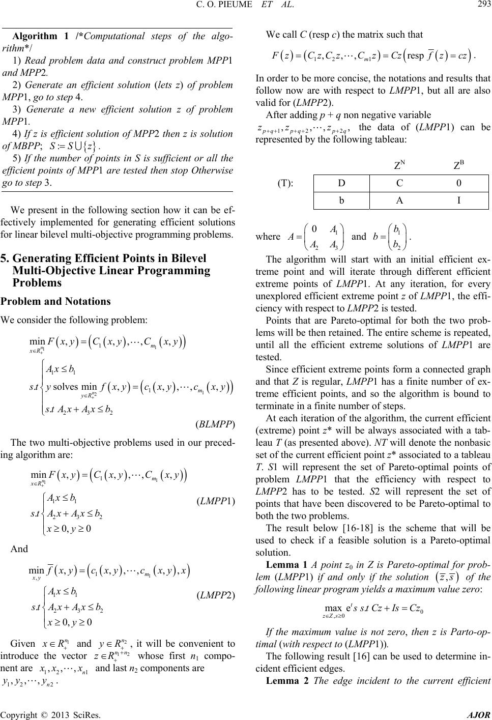 C. O. PIEUME ET AL. 293 Algorithm 1 /*Computational steps of the algo- rithm*/ 1) Read problem data and construct problem MPP1 and MPP 2. 2) Generate an efficient solution (lets z) of problem MPP1, go to step 4. 3) Generate a new efficient solution z of problem MPP1. 4) If z is efficient solution of MPP2 then z is solution of MBPP; . :SS z 5) If the number of points in S is sufficient or all the efficient points of MPP1 are tested then stop Otherwise go to step 3. We present in the following section how it can be ef- fectively implemented for generating efficient solutions for linear bilevel multi-objective programming problems. 5. Generating Efficient Points in Bilevel Multi-Objective Linear Programming Problems Problem and Notations We consider the following problem: 1 1 2 1 11 1 232 min,,,,, .solvesmin ,, . n n m xR yR FxyCxyCxy Ax b 1 ,, , m tyfxycxy st AxAxb c xy 1 , , m (BLMPP) The two multi-objective problems used in our preced- ing algorithm are: 11 11 232 min,, , . 0, 0 n xR xyC xy Ax b st AxAxb xy C xy (LMPP1) And 1 , 11 232 min,, , . 0, 0 xy 1 ,, , m xyc xy Ax b st AxAxb xy cxyx 2 n yR (LMPP2) Given and 1 n xR 12 nn zR 1 , n , it will be convenient to introduce the vector whose first n1 compo- nent are 12 ,, x ,yx 12 2n and last n2 components are ,,yy. We call C (resp c) the matrix such that 12 1 ,,, resp m zCzCzCzCz fzcz ,,,,zz z . In order to be more concise, the notations and results that follow now are with respect to LMPP1, but all are also valid for (LMPP2). After adding p + q non negative variable 12 2pqpqp q the data of (LMPP1) can be represented by the following tableau: Z N ZB (T): D C 0 b A I 1 23 0 where A A 1 2 b bb and . The algorithm will start with an initial efficient ex- treme point and will iterate through different efficient extreme points of LMPP1. At any iteration, for every unexplored efficient extreme point z of LMPP1, the effi- ciency with respect to LMPP2 is tested. Points that are Pareto-optimal for both the two prob- lems will be then retained. The entire scheme is repeated, until all the efficient extreme solutions of LMPP1 are tested. Since efficient extreme points form a connected graph and that Z is regular, LMPP1 has a finite number of ex- treme efficient points, and so the algorithm is bound to terminate in a finite number of steps. At each iteration of the algorithm, the current efficient (extreme) point z* will be always associated with a tab- leau T (as presented above). NT will denote the nonbasic set of the current efficient point z* associated to a tableau T. S1 will represent the set of Pareto-optimal points of problem LMPP1 that the efficiency with respect to LMPP2 has to be tested. S2 will represent the set of points that have been discovered to be Pareto-optimal to both the two problems. The result below [16-18] is the scheme that will be used to check if a feasible solution is a Pareto-optimal solution. Lemma 1 A point z0 in Z is Pareto-optimal for prob- lem (LMPP1) if and only if the solution ,zs 0 ,0 max e. t zZs of the following linear program yields a maxim um value zero: stCz IsCz If the maximum value is not zero, then z is Parto-op- timal (with respect to (LMPP1)). The following result [16] can be used to determine in- cident efficient edges. Lemma 2 The edge incident to the current efficient Copyright © 2013 SciRes. AJOR 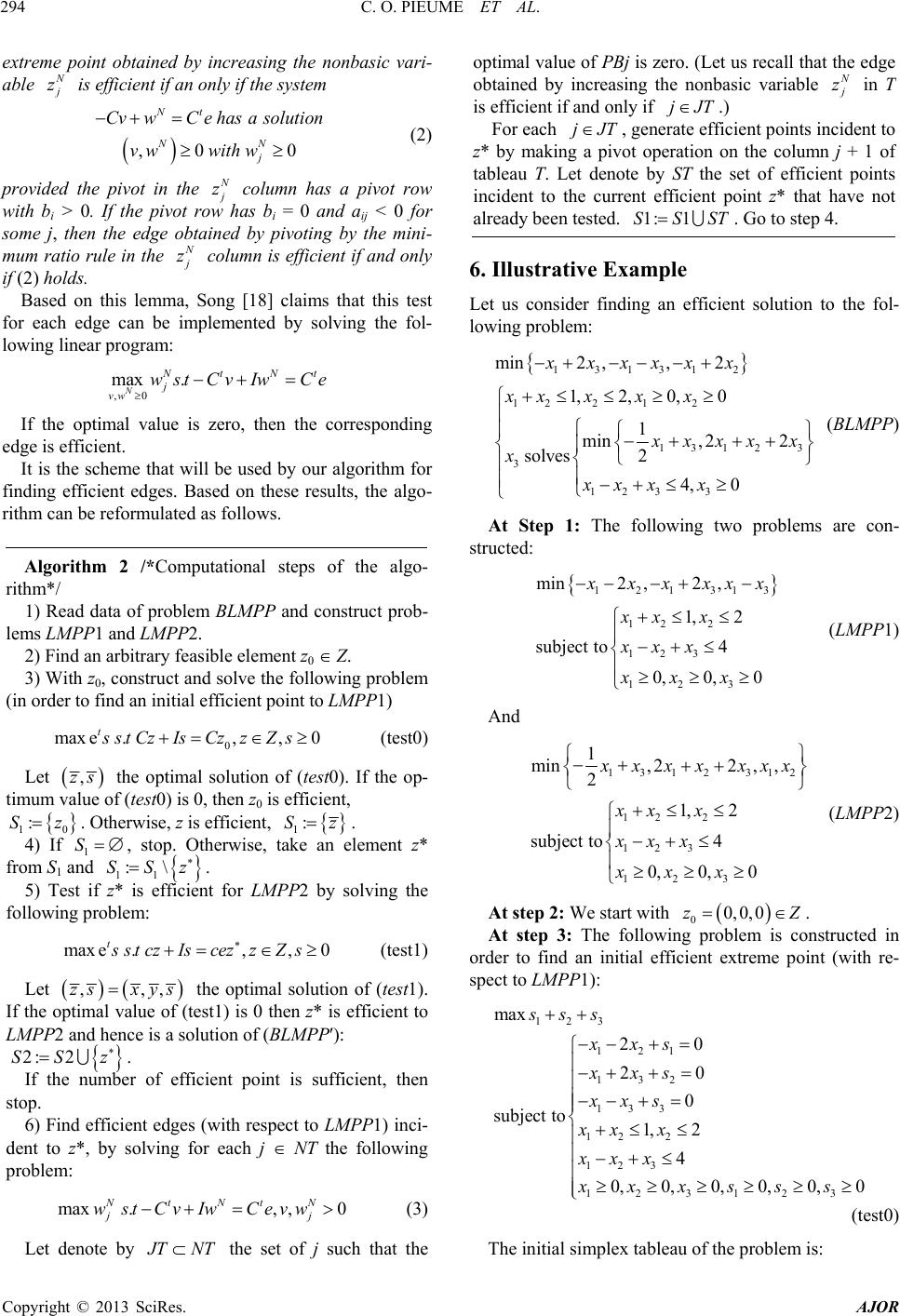 C. O. PIEUME ET AL. 294 extreme point obtained by increasing the nonbasic vari- able z 0 N j has a solution wth is efficient if an only if the system ,0 Nt N CvwC e vw wi (2) provided the pivot in the z column has a pivot row with bi > 0. If the pivot row has bi = 0 and aij < 0 for some j, then the edge obtained by pivoting by the mini- mum ratio rule in the z Nt vIwCe column is efficient if and only if (2) holds. Based on this lemma, Song [18] claims that this test for each edge can be implemented by solving the fol- lowing linear program: ,0 .max N Nt j vw stwC If the optimal value is zero, then the corresponding edge is efficient. It is the scheme that will be used by our algorithm for finding efficient edges. Based on these results, the algo- rithm can be reformulated as follows. Algorithm 2 /*Computational steps of the algo- rithm*/ 1) Read data of problem BLMPP and construct prob- lems LMPP1 and LMPP2. 2) Find an arbitrary feasible element z0 Z. 3) With z0, construct and solve the following proble (in order to find an initial efficient point to LMPP1) 0, 0,zZ s max e. tsstCzIsCz (test0) Let ,zs 1 :Sz the optimal solution of (test0). If the op- timum value of (test0) is 0, then z0 is efficient, . Otherwise, z is efficient, 0 :Sz S :\SSz ,, 0zzZs 1 4) If 1, stop. Otherwise, take an element z* from S1 and . . 11 5) Test if z* is efficient for LMPP2 by solving the following problem: max e. tsstczIsce (test1) Let ,,,zs xys 2SSz the optimal solution of (test1). If the optimal value of (test1) is 0 then z* is efficient to LMPP2 and hence is a solution of (BLMPP′): . 2: If the number of efficient point is sufficient, the stop. 6) Find efficient edges (with respect to LMPP1) inci- dent to z*, by solving for each j NT the following problem: .max NtN wCvIst w ,,0 tN jj Ce v w (3) Let denote by TNT the set of j such that the optimal value of PBj is zero. (Let us recall that the edge obtained by increasing the nonbasic variable z in is efficient if and only if jJT .) For each jJT , generate efficient points incident to z* by making a pivot operation on the column j + 1 o tableau T. Let denote by ST the set of efficient points incident to the current efficient point z* that have no already been tested. 1: 1SSST. Go to step 4. 6. Illustrative Example Let us consider finding an efficient solution to the fol- lowing problem: 131312 12212 1312 3 3 123 3 min 22 1,2, 0,0 1 min, 22 2 solves , 4, 0 ,xxxxxx xx xxx xxx x x xxx x (BLMPP) At Step 1: The following two problems are con- structed: 121313 12 2 123 123 min2 ,2 , 1, 2 subject to4 0,0, 0 xx xxx xx x xxx xxx (LMPP1) And 1312 312 12 2 123 123 1 min, 22,, 2 1, 2 subject to4 0,0, 0 xxxxxx xx x xxx xxx 0, 0,0zZ 123 121 132 133 12 2 123 123123 max 20 20 0 subject to1, 2 4 0,0,0, 0,0,0 sss xxs xxs xxs xx x xxx xxxsss (LMPP2) At step 2: We start with . 0 At step 3: The following problem is constructed in order to find an initial efficient extreme point (with re- spect to LMPP1): (test0) The initial simplex tableau of the problem is: Copyright © 2013 SciRes. AJOR 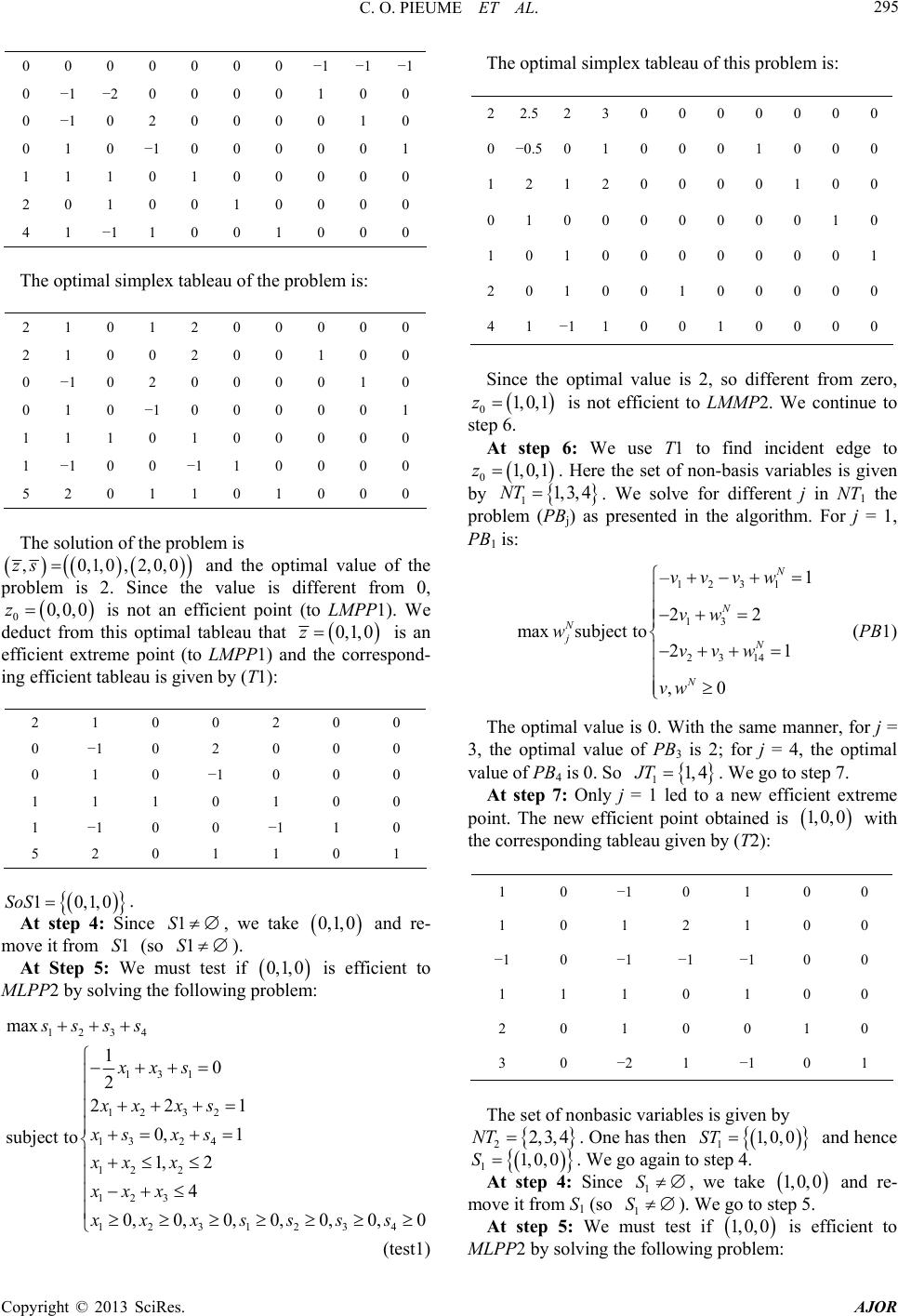 C. O. PIEUME ET AL. 295 Copyright © 2013 SciRes. AJOR 0 0 0 0 0 0 0 −1 −1−1 0 −1 −2 0 0 0 0 1 0 0 0 −1 0 2 0 0 0 0 1 0 0 1 0 −1 0 0 0 0 0 1 1 1 1 0 1 0 0 0 0 0 2 0 1 0 0 1 0 0 0 0 4 1 −1 1 0 0 1 0 0 0 The optimal simplex tableau of the problem is: 2 1 0 1 2 0 0 0 0 0 2 1 0 0 2 0 0 1 0 0 0 −1 0 2 0 0 0 0 1 0 0 1 0 −1 0 0 0 0 0 1 1 1 1 0 1 0 0 0 0 0 1 −1 0 0 −1 1 0 0 0 0 5 2 0 1 1 0 1 0 0 0 The solution of the problem is 0,1,zs , 0,20,0, and the optimal value of the problem is 2. Since the value is different from 0, 0 is not an efficient point (to LMPP1). We deduct from this optimal tableau that 0, 0, 0z 0,1, 0z is an efficient extreme point (to LMPP1) and the correspond- ing efficient tableau is given by (T1): 2 1 0 0 2 0 0 0 −1 0 2 0 0 0 0 1 0 −1 0 0 0 1 1 1 0 1 0 0 1 −1 0 0 −1 1 0 5 2 0 1 1 0 1 10,1,0 1S SoS . At step 4: Since , we take 0,1,0 1 and re- move it from (so S). 1S At Step 5: We must test if 0,1,0 is efficient to MLPP2 by solving the following problem: 1234 131 12 32 13 24 12 2 123 12 31 max 10 2 221 0, 1 subject to 1, 2 4 0,0,0, 0,0, ssss xxs xx xs xs xs xx x xxx xxxss 234 0, 0ss (test1) The optimal simplex tableau of this problem is: 2 2.52 3 0 0 0 0 0 0 0 0 −0.50 1 0 0 0 1 0 0 0 1 2 1 2 0 0 0 0 1 0 0 0 1 0 0 0 0 0 0 0 1 0 1 0 1 0 0 0 0 0 0 0 1 2 0 1 0 0 1 0 0 0 0 0 4 1 −11 0 0 1 0 0 0 0 Since the optimal value is 2, so different from zero, 0 is not efficient to LMMP2. We continue to step 6. 1,0, 1z At step 6: We use T1 to find incident edge to 0. Here the set of non-basis variables is given by 1,0, 1z 1, 3,4NT 123 1 13 23 14 –1 22 maxsubject to 21 ,0 N N N jN N vvvw vw wvvw vw 1. We solve for different j in NT1 the problem (PBj) as presented in the algorithm. For j = 1, PB1 is: (PB1) The optimal value is 0. With the same manner, for j = 3, the optimal value of PB3 is 2; for j = 4, the optimal value of PB4 is 0. So 1 At step 7: Only j = 1 led to a new efficient extreme point. The new efficient point obtained is 1, 4JT . We go to step 7. 1, 0,0 with the corresponding tableau given by (T2): 1 0 −1 0 1 0 0 1 0 1 2 1 0 0 −1 0 −1 −1 −1 0 0 1 1 1 0 1 0 0 2 0 1 0 0 1 0 3 0 −2 1 −1 0 1 The set of nonbasic variables is given by 22,3,4NT 1, 0, 0ST . One has then 1 and hence 11, 0, 0S 1 S . We go again to step 4. At step 4: Since , we take 1, 0, 0 S and re- move it from S1 (so 1 ). We go to step 5. At step 5: We must test if 1, 0, 0 is efficient to MLPP2 by solving the following problem: 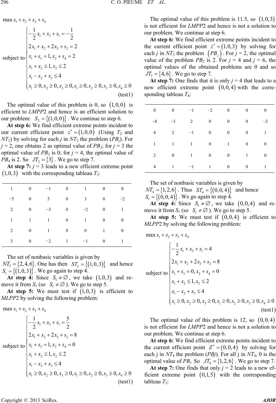 C. O. PIEUME ET AL. 296 1234 131 12 32 132 4 12 2 123 12 31 max 11 22 222 1, 2 subject to 1, 2 4 0,0,0, 0,0, ssss xxs xx xs xs xs xx x xxx xxxss 234 0, 0ss (test1) The optimal value of this problem is 0, so 1, 0,0 1, 0, 0 1, 0, 0z is efficient to LMPP2 and hence is an efficient solution to our problem: . We continue to step 6. 2 At step 6: We find efficient extreme points incident to our current efficient point (Using T2 and NT2) by solving for each j in NT2 the problem (PBj). For j = 2, one obtains 2 as optimal value of PB2; for j = 3 the optimal value of PB3 is 0; for j = 4, the optimal value of PB4 is 2. So S 23JT . We go to step 7. At step 7: j = 3 leads to a new efficient extreme point with the corresponding tableau T3: 1, 0, 3 1 0 −1 0 1 0 0 −5 0 5 0 3 0 −2 2 0 −3 0 −2 0 1 1 1 1 0 1 0 0 2 0 1 0 0 1 0 3 0 −2 1 −1 0 1 The set of nonbasic variables is given by . One has then 32, 4, 6NT 2 and hence 1, 0, 3 ST 11, 0, 3S. We go again to step 4. At step 4: Since , we take 1 S 1, 0, 3 S and re- move it from S1 (so ). We go to step 5. 1 At step 5: We must test if 1, 0, 3 is efficient to MLPP2 by solving the following problem: 1234 131 12 32 132 4 12 2 123 12 31 max 15 22 228 1, 0 subject to 1, 2 4 0,0,0, 0,0, ssss xxs xx xs xs xs xx x xxx xxxss The optimal value of this problem is 11.5, so 1, 0,3 is not efficient for LMPP2 and hence is not a solution to our problem. We continue at step 6. At step 6: We find efficient extreme points incident to the current efficient point 1, 0, 3z by solving for each j in NT3 the problem j. For j = 2, the optimal value of the problem PB2 is 2. For j = 4 and j = 6, the optimal values of the obtained problems are 0 and so PB 3 At step 7: One finds that it is only j = 4 that leads to a new efficient extreme point 4, 6JT . We go to step 7. 0, 0, 4with the corre- sponding tableau T4: 0 0 −1 −2 0 0 0 −8 −3 2 0 0 0 −2 4 2 −1 0 0 0 1 1 1 1 0 1 0 0 2 0 1 0 0 1 0 4 1 −1 1 0 0 1 The set of nonbasic variables is given by 41, 2,6NT 0, 0, 4ST . Thus 4 and hence 10, 0, 4S 1 S . We go again to step 4. At step 4: Since 0, 0, 4 S, we take and re- move it from S1 (so 234 0, 0ss (test1) 1 0, 0, 4 ). We go to step 5. At step 5: We must test if is efficient to MLPP2 by solving the following problem: 12 34 131 12 32 13 24 12 2 123 1231234 max 14 2 228 0, 0 subject to 1, 2 4 0,0,0,0, 0,0, 0 ssss xxs xx xs xs xs xx x xxx xxxssss (test1) The optimal value of this problem is 12, so 0, 0, 4 is not efficient for LMPP2 and hence is not a solution to our problem. We continue at step 6. At step 6: We find efficient extreme points incident to the current efficient point 0, 0, 4Z by solving for each j in NT4 the problem (PBj). For all j in NT4, 0 is the optimal value of PBj. So 4 At step 7: One finds that only j = 2 leads to a new ef- ficient extreme point 1, 2,6JT. We go to step 7. 0,1,5 with the corresponding tableau T5: Copyright © 2013 SciRes. AJOR 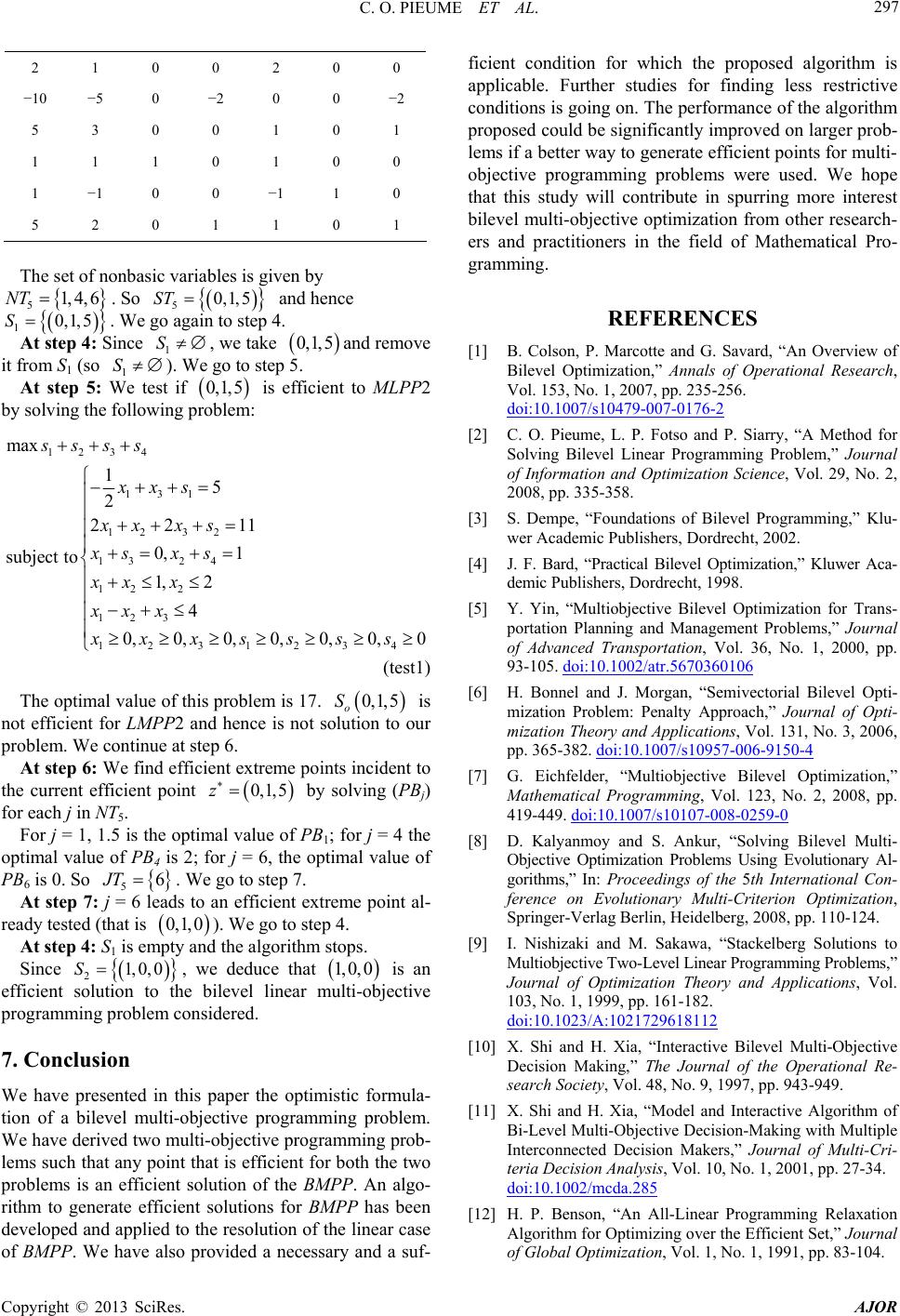 C. O. PIEUME ET AL. 297 2 1 0 0 2 0 0 −10 −5 0 −2 0 0 −2 5 3 0 0 1 0 1 1 1 1 0 1 0 0 1 −1 0 0 −1 1 0 5 2 0 1 1 0 1 The set of nonbasic variables is given by 5 NT 1, 4,6 . So 5 and hence ST 0, 1,5 1 0,1,5 S S. We go again to step 4. At step 4: Since 1, we take 0,1,5 S and remove it from S1 (so ). We go to step 5. 1 At step 5: We test if 0,1,5 is efficient to MLPP2 by solving the following problem: 1234 131 12 32 13 24 12 2 123 12 31 max 15 2 2211 0, 1 subject to 1, 2 4 0,0,0, 0,0, ssss xxs xx xs xs xs xx x xxx xxxss 234 0, 0ss (test1) The optimal value of this problem is 17. 0,1,5S o is not efficient for LMPP2 and hence is not solution to our problem. We continue at step 6. At step 6: We find efficient extreme points incident to the current efficient point 0,1,5z by solving (PBj) for each j in NT5. For j = 1, 1.5 is the optimal value of PB1; for j = 4 the optimal value of PB4 is 2; for j = 6, the optimal value of PB6 is 0. So 5 At step 7: j = 6 leads to an efficient extreme point al- ready tested (that is 6JT . We go to step 7. 0,1,0 1, 0, 0 ). We go to step 4. At step 4: S1 is empty and the algorithm stops. Since 2, we deduce that S 1, 0, 0 is an efficient solution to the bilevel linear multi-objective programming problem considered. 7. Conclusion We have presented in this paper the optimistic formula- tion of a bilevel multi-objective programming problem. We have derived two multi-objective programming prob- lems such that any point that is efficient for both the two problems is an efficient solution of the BMPP. An algo- rithm to generate efficient solutions for BMPP has been developed and applied to the resolution of the linear case of BMPP. We have also provided a necessary and a suf- ficient condition for which the proposed algorithm is applicable. Further studies for finding less restrictive conditions is going on. The performance of the algorithm proposed could be significantly improved on larger prob- lems if a better way to generate efficient points for multi- objective programming problems were used. We hope that this study will contribute in spurring more interest bilevel multi-objective optimization from other research- ers and practitioners in the field of Mathematical Pro- gramming. REFERENCES [1] B. Colson, P. Marcotte and G. Savard, “An Overview of Bilevel Optimization,” Annals of Operational Research, Vol. 153, No. 1, 2007, pp. 235-256. doi:10.1007/s10479-007-0176-2 [2] C. O. Pieume, L. P. Fotso and P. Siarry, “A Method for Solving Bilevel Linear Programming Problem,” Journal of Information and Optimization Science, Vol. 29, No. 2, 2008, pp. 335-358. [3] S. Dempe, “Foundations of Bilevel Programming,” Klu- wer Academic Publishers, Dordrecht, 2002. [4] J. F. Bard, “Practical Bilevel Optimization,” Kluwer Aca- demic Publishers, Dordrecht, 1998. [5] Y. Yin, “Multiobjective Bilevel Optimization for Trans- portation Planning and Management Problems,” Journal of Advanced Transportation, Vol. 36, No. 1, 2000, pp. 93-105. doi:10.1002/atr.5670360106 [6] H. Bonnel and J. Morgan, “Semivectorial Bilevel Opti- mization Problem: Penalty Approach,” Journal of Opti- mization Theory and Applications, Vol. 131, No. 3, 2006, pp. 365-382. doi:10.1007/s10957-006-9150-4 [7] G. Eichfelder, “Multiobjective Bilevel Optimization,” Mathematical Programming, Vol. 123, No. 2, 2008, pp. 419-449. doi:10.1007/s10107-008-0259-0 [8] D. Kalyanmoy and S. Ankur, “Solving Bilevel Multi- Objective Optimization Problems Using Evolutionary Al- gorithms,” In: Proceedings of the 5th International Con- ference on Evolutionary Multi-Criterion Optimization, Springer-Verlag Berlin, Heidelberg, 2008, pp. 110-124. [9] I. Nishizaki and M. Sakawa, “Stackelberg Solutions to Multiobjective Two-Level Linear Programming Problems,” Journal of Optimization Theory and Applications, Vol. 103, No. 1, 1999, pp. 161-182. doi:10.1023/A:1021729618112 [10] X. Shi and H. Xia, “Interactive Bilevel Multi-Objective Decision Making,” The Journal of the Operational Re- search Society, Vol. 48, No. 9, 1997, pp. 943-949. [11] X. Shi and H. Xia, “Model and Interactive Algorithm of Bi-Level Multi-Objective Decision-Making with Multiple Interconnected Decision Makers,” Journal of Multi-Cri- teria Decision Analysis, Vol. 10, No. 1, 2001, pp. 27-34. doi:10.1002/mcda.285 [12] H. P. Benson, “An All-Linear Programming Relaxation Algorithm for Optimizing over the Efficient Set,” Journal of Global Optimization, Vol. 1, No. 1, 1991, pp. 83-104. Copyright © 2013 SciRes. AJOR  C. O. PIEUME ET AL. Copyright © 2013 SciRes. AJOR 298 doi:10.1007/BF00120667 [13] M. Ehrgott, “Multicriteria Optimisation,” Springer, Berlin, 2000. [14] H. Iserman, “The Enumeration of the Set of All Efficient Solutions for a Linear Multiple Objective Program,” Op- erational Research Quarterly, Vol. 28, No. 3, 1977, pp. 711-725. [15] C. O. Pieume, L. P. Fotso and P. Siarry, “Finding Effi- cient Set in Multiobjective Linear Programming,” Journal of Information and Optimization Science, Vol. 29, No. 2, 2008, pp. 203-216. [16] J. G. Ecker, N. S. Hegner and I. A. Kouada, “Generating All Maximal Efficient Faces for Multiple Objective Lin- ear Programs,” Journal of Optimisation Theory and Ap- plications, Vol. 30, No. 3, 1980, pp. 353-381. doi:10.1007/BF00935493 [17] Y. Yamamoto, “Optimization over the Efficient Set: Over- view,” Journal of Global Optimization, Vol. 22, No. 1-4, 2002, pp. 285-317. doi:10.1023/A:1013875600711 [18] J. G. Ecker and J. H. Song, “Optimizing a Linear Func- tion over an Efficient Set,” Journal of Optimization The- ory and Applications, Vol. 83, No. 3, 1994, pp. 541-563. doi:10.1007/BF02207641
|