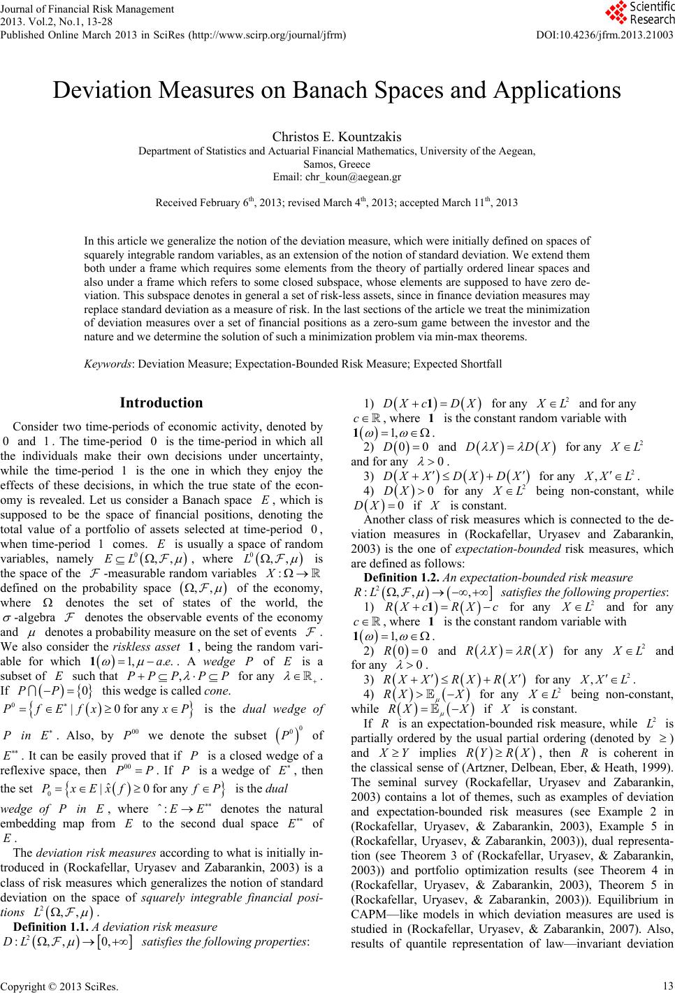
 Journal of Financial Risk Management 2013. Vol.2, No.1, 13-28 Published Online March 2013 in SciRes (http://www.scirp.org/journal/jfrm) DOI:10.4236/jfrm.2013.21003 Deviation Measures on Banach Spaces and Applications Christos E. Kountzakis Department of Statistics and Actuarial Financial Mathematics, University of the Aegean, Samos, Greece Email: chr_koun@aegean.gr Received February 6th, 2013; revised March 4th, 2013; accepted March 11th, 2013 In this article we generalize the notion of the deviation measure, which were initially defined on spaces of squarely integrable random variables, as an extension of the notion of standard deviation. We extend them both under a frame which requires some elements from the theory of partially ordered linear spaces and also under a frame which refers to some closed subspace, whose elements are supposed to have zero de- viation. This subspace denotes in general a set of risk-less assets, since in finance deviation measures may replace standard deviation as a measure of risk. In the last sections of the article we treat the minimization of deviation measures over a set of financial positions as a zero-sum game between the investor and the nature and we determine the solution of such a minimization problem via min-max theorems. Keywords: Deviation Measure; Expectation-Bounded Risk Measure; Expected Shortfall Introduction Consider two time-periods of economic activity, denoted by and 1. The time-period is the time-period in which all the individuals make their own decisions under uncertainty, while the time-period is the one in which they enjoy the effects of these decisions, in which the true state of the econ- omy is revealed. Let us consider a Banach space , which is supposed to be the space of financial positions, denoting the total value of a portfolio of assets selected at time-period , when time-period comes. is usually a space of random variables, namely 00 E 1 E 0 1 0,,EL , where 0,,L X : is the space of the -measurable random variables defined on the probability space ,, of the economy, where denotes the set of states of the world, the -algebra denotes the observable events of the economy and denotes a probability measure on the set of events . We also consider the riskless asset , being the random vari- able for which 1. A wedge of is a subset of such that 1 ,P 1, . PP.ae P E EP P for any . If 0 PP this wedge is called cone. 0|E 0 for anxyPf fxP is the dual wedge of in . Also, by we denote the subset of PE00 P 0 0 P E. It can be easily proved that if is a closed wedge of a reflexive space, then . If is a wedge of P P 00 PPE , then the set 0ˆ |0for anyPxExf fP is the dual wedge of in , where denotes the natural embedding map from to the second dual space P Eˆ :EE EE of . E The deviation risk measures according to what is initially in- troduced in (Rockafellar, Uryasev and Zabarankin, 2003) is a class of risk measures which generalizes the notion of standard deviation on the space of squarely integrable financial posi- tions 2,,L . Definition 1.1. A deviation risk measure 2 :,, 0,DL 1) DX cDX1 for any 2 L and for any c , where is the constant random variable with 1 1, 1. 2) 00D and DX DX for any 2 L and for any 0 . 3) DX XDXDX for any 2 , XL . 4) 0DX 2 for any L being non-constant, while 0DX if is constant. Another class of risk measures which is connected to the de- viation measures in (Rockafellar, Uryasev and Zabarankin, 2003) is the one of expectation-bounded risk measures, which are defined as follows: Definition 1.2. An expectation-bounded risk measure 2 :,, ,RL satisfies the following properties: 1) RX cRXc 1 for any 2 L and for any c , where is the constant random variable with 1 1, 1. 2) 00R and RX RX for any 2 L and for any 0 . 3) X XRXRX for any 2 L ,XX . 4) RX X for any 2 L being non-constant, while X X if is constant. X If is an expectation-bounded risk measure, while 2 is partially ordered by the usual partial ordering (denoted by ) and implies XY YRX, then is coherent in the classical sense of (Artzner, Delbean, Eber, & Heath, 1999). The seminal survey (Rockafellar, Uryasev and Zabarankin, 2003) contains a lot of themes, such as examples of deviation and expectation-bounded risk measures (see Example 2 in (Rockafellar, Uryasev, & Zabarankin, 2003), Example 5 in (Rockafellar, Uryasev, & Zabarankin, 2003)), dual representa- tion (see Theorem 3 of (Rockafellar, Uryasev, & Zabarankin, 2003)) and portfolio optimization results (see Theorem 4 in (Rockafellar, Uryasev, & Zabarankin, 2003), Theorem 5 in (Rockafellar, Uryasev, & Zabarankin, 2003)). Equilibrium in CAPM—like models in which deviation measures are used is studied in (Rockafellar, Uryasev, & Zabarankin, 2007). Also, results of quantile representation of law—invariant deviation satisfies the following properties: Copyright © 2013 SciRes. 13 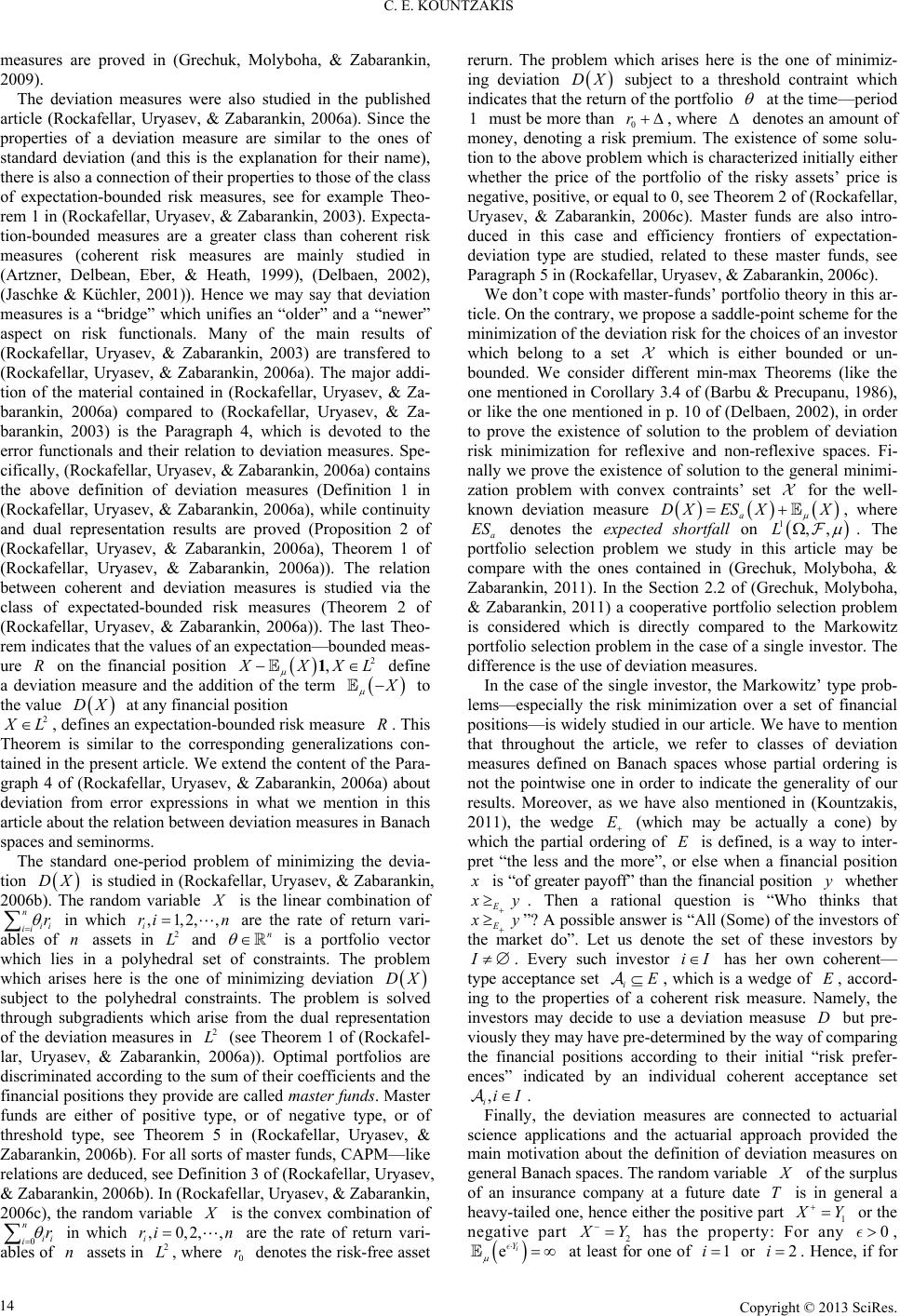 C. E. KOUNTZAKIS measures are proved in (Grechuk, Molyboha, & Zabarankin, 2009). The deviation measures were also studied in the published article (Rockafellar, Uryasev, & Zabarankin, 2006a). Since the properties of a deviation measure are similar to the ones of standard deviation (and this is the explanation for their name), there is also a connection of their properties to those of the class of expectation-bounded risk measures, see for example Theo- rem 1 in (Rockafellar, Uryasev, & Zabarankin, 2003). Expecta- tion-bounded measures are a greater class than coherent risk measures (coherent risk measures are mainly studied in (Artzner, Delbean, Eber, & Heath, 1999), (Delbaen, 2002), (Jaschke & Küchler, 2001)). Hence we may say that deviation measures is a “bridge” which unifies an “older” and a “newer” aspect on risk functionals. Many of the main results of (Rockafellar, Uryasev, & Zabarankin, 2003) are transfered to (Rockafellar, Uryasev, & Zabarankin, 2006a). The major addi- tion of the material contained in (Rockafellar, Uryasev, & Za- barankin, 2006a) compared to (Rockafellar, Uryasev, & Za- barankin, 2003) is the Paragraph 4, which is devoted to the error functionals and their relation to deviation measures. Spe- cifically, (Rockafellar, Uryasev, & Zabarankin, 2006a) contains the above definition of deviation measures (Definition 1 in (Rockafellar, Uryasev, & Zabarankin, 2006a), while continuity and dual representation results are proved (Proposition 2 of (Rockafellar, Uryasev, & Zabarankin, 2006a), Theorem 1 of (Rockafellar, Uryasev, & Zabarankin, 2006a)). The relation between coherent and deviation measures is studied via the class of expectated-bounded risk measures (Theorem 2 of (Rockafellar, Uryasev, & Zabarankin, 2006a)). The last Theo- rem indicates that the values of an expectation—bounded meas- ure on the financial position 2 , XXL 1 define a deviation measure and the addition of the term to the value at any financial position DX 2 L, defines an expectation-bounded risk measure . This Theorem is similar to the corresponding generalizations con- tained in the present article. We extend the content of the Para- graph 4 of (Rockafellar, Uryasev, & Zabarankin, 2006a) about deviation from error expressions in what we mention in this article about the relation between deviation measures in Banach spaces and seminorms. The standard one-period problem of minimizing the devia- tion is studied in (Rockafellar, Uryasev, & Zabarankin, 2006b). The random variable is the linear combination of ii DX ii rX n in which i are the rate of return vari- ables of assets in ,1,2ri 2 ,,n n and is a portfolio vector which lies in a polyhedral set of constraints. The problem which arises here is the one of minimizing deviation n DX subject to the polyhedral constraints. The problem is solved through subgradients which arise from the dual representation of the deviation measures in 2 (see Theorem 1 of (Rockafel- lar, Uryasev, & Zabarankin, 2006a)). Optimal portfolios are discriminated according to the sum of their coefficients and the financial positions they provide are called master funds. Master funds are either of positive type, or of negative type, or of threshold type, see Theorem 5 in (Rockafellar, Uryasev, & Zabarankin, 2006b). For all sorts of master funds, CAPM—like relations are deduced, see Definition 3 of (Rockafellar, Uryasev, & Zabarankin, 2006b). In (Rockafellar, Uryasev, & Zabarankin, 2006c), the random variable is the convex combination of 0 i X n ii r in which i are the rate of return vari- ables of assets in ,0,ri 2 2,,n n , where denotes the risk-free asset rerurn. The problem which arises here is the one of minimiz- ing deviation 0 r DX subject to a threshold contraint which indicates that the return of the portfolio at the time—period must be more than 0 1r , where denotes an amount of money, denoting a risk premium. The existence of some solu- tion to the above problem which is characterized initially either whether the price of the portfolio of the risky assets’ price is negative, positive, or equal to 0, see Theorem 2 of (Rockafellar, Uryasev, & Zabarankin, 2006c). Master funds are also intro- duced in this case and efficiency frontiers of expectation- deviation type are studied, related to these master funds, see Paragraph 5 in (Rockafellar, Uryasev, & Zabarankin, 2006c). We don’t cope with master-funds’ portfolio theory in this ar- ticle. On the contrary, we propose a saddle-point scheme for the minimization of the deviation risk for the choices of an investor which belong to a set which is either bounded or un- bounded. We consider different min-max Theorems (like the one mentioned in Corollary 3.4 of (Barbu & Precupanu, 1986), or like the one mentioned in p. 10 of (Delbaen, 2002), in order to prove the existence of solution to the problem of deviation risk minimization for reflexive and non-reflexive spaces. Fi- nally we prove the existence of solution to the general minimi- zation problem with convex contraints’ set for the well- known deviation measure a SDXX X E, where a S denotes the expected shortfall on 1 L,, . The portfolio selection problem we study in this article may be compare with the ones contained in (Grechuk, Molyboha, & Zabarankin, 2011). In the Section 2.2 of (Grechuk, Molyboha, & Zabarankin, 2011) a cooperative portfolio selection problem is considered which is directly compared to the Markowitz portfolio selection problem in the case of a single investor. The difference is the use of deviation measures. In the case of the single investor, the Markowitz’ type prob- lems—especially the risk minimization over a set of financial positions—is widely studied in our article. We have to mention that throughout the article, we refer to classes of deviation measures defined on Banach spaces whose partial ordering is not the pointwise one in order to indicate the generality of our results. Moreover, as we have also mentioned in (Kountzakis, 2011), the wedge (which may be actually a cone) by which the partial ordering of is defined, is a way to inter- pret “the less and the more”, or else when a financial position is “of greater payoff” than the financial position whether y E y . Then a rational question is “Who thinks that E y ”? A possible answer is “All (Some) of the investors of the market do”. Let us denote the set of these investors by I . Every such investor has her own coherent— type acceptance set i iI , which is a wedge of , accord- ing to the properties of a coherent risk measure. Namely, the investors may decide to use a deviation measuse but pre- viously they may have pre-determined by the way of comparing the financial positions according to their initial “risk prefer- ences” indicated by an individual coherent acceptance set D , iiI . Finally, the deviation measures are connected to actuarial science applications and the actuarial approach provided the main motivation about the definition of deviation measures on general Banach spaces. The random variable of the surplus of an insurance company at a future date is in general a heavy-tailed one, hence either the positive part 1 X T Y or the negative part 2 Y has the property: For any , 0 ei Y at least for one of or . Hence, if for 1i2i Copyright © 2013 SciRes. 14  C. E. KOUNTZAKIS example for the maximum for which p p X , holds, then 1p ,,EL p may be naturally considered as the Banach space of the surplus positions, if the distribution of is such that leads to this result. Another motivation for this generalization is the actuarial definition of Solvency Capital, as it is mentioned in (Dhaene, Goovaerts, Kaas, Tang, Vanduffel, & Vyncke, 2003). In this review on risk measures and the notion of solvency the following definition of capital requirement functional for an insurance company is given: if represents the time-T liabilities of an insurance company and X X X is the economic capital associated with these liabilites, while is the value of them calculated either by a quantile method, or by an additional margin method, or by a replicationg portfolio method, then if the risk measure used is PX , the solvency capital for is equal to X . The functionals , P are connected to by the identity KX PX P for any which is a liability vari- able. If X , or else the pricing functional is considered without the margin term, then we may take that K . If is a coherent risk measure, then is a deviation measure. In these case the insurance company calculates its own Sol- vency Capital with respect to a generalized risk measure (for example a deviation one), so that it may be acceptable by the regulator. Since the liability variable is a heavy-tail dis- X tributed one, the moments X p L exist till a specific value of . If , we may consider p1p ,, or 1 to be the model in which we work. This is a motivation for the use of deviation measures on Banach spaces except 2 . Another motivation related to financial applications is the class of G -spaces, which are actually Banach spaces related to G-expectation, see in (Peng, 2007). We may suppose that the variables which denote the value of the portfolios at a certain future date , belong to such spaces, since martingale theory according to the G-expectation is related to the T 2 G space, as (Soner, Touzi, & Zhang, 2011) indicates. Hence, we may con- sider the case of definition of deviation measures on this class of Banach spaces. Also, a reference about considering stochas- tic models of markets under model uncertainty is (Denis & Martini, 2006). But the definition and the study of deviation measures on G -spaces should require a separate article. Deviation Measures on Banach Spaces First we remind the definitions of convex and coherent risk measures associated to the Monotonocity property related to the partial ordering defined on by some wedge of it. In the following we refer to the notions of the , e-co- herent and , e-convex risk measures (where is par- tially ordered by the partial ordering relation induced by the wedge E of it), whose definitions are the following: Definition 2.1. A function :E , which satis- fies the properties 1) ae x a (e-Translation Invariance). 2) 11 xx y for any 0,1 A y (Convexity). 3) implies x yx ( -Monotonicity). where , yE is called , e -convex risk measure. Definition 2.2. A function :E , is a , e- coherent risk measure if it is an , e-convex risk measure and it satisfies the following property: x for any E and any (Positive Homogeneity). In both of these definitions, we suppose that I , be- ing the characteristic function of the value . Let be a Banach space, being partially ordered by a closed cone of . Also consider a non-trivial, closed subspace EP E of . Suppose that this cone has a base E defined by a continuous linear functional of , namely that E |1xBxP Definition 2.3. A . -deviation risk measure :0,DE satisfies the following properties: 1) Dx ctDx for any E and for any c and any tKB 2) . 0D0 and Dx Dx for any E and for any 0 . 3) Dx xDxDx for any , xE . 4) 0Dx for any EK, while 0Dx if K . The definition of the -expectation-bounded risk measures is the following: Definition 2.4. A -expectation-bounded risk measure :,RE satisfies the following properties: 1) RxcRx ce for any E and for any c and any eKB . 2) 0R0 and xR x for any E and for any 0 . 3) x xRxRx for any , xE . 4) xRx for any EK, while xRx if K . If is a -expectation-bounded risk measure, while is partially ordered by the usual partial ordering induced by (denoted by P) and E P P y implies yRx, then is ,Pe -coherent. Proposition 2.5. If is a -deviation measure on D K , the functional :, D RE , where ,, DxxxE Rx D is a -expectation bounded risk measure. K Proof. It suffices to prove that satisfies the properties of a -expectation bounded risk measure on the partially or- dered Banach space . E 1) DD xctRxc for any E and for any ,ctKB . This property holds due to the definition of and the equivalent property of , which is a -devia- tion measure, namely D K . D Rxx ctx ct Dxxct Rx c D ct D 2) 00 D R and DD xRx for any E and for any 0 . This property also holds due to the definition of and the equivalent property of as a deviation measure, namely D 00RD 00 D and , DD xDDxx Rx x x if 0 and for any E . 3) DDD xxxRxR for any , xE . By the same way, we have that Dx Dx D Rxxx xx Dxxx , Copyright © 2013 SciRes. 15 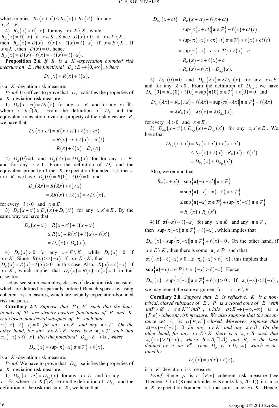 C. E. KOUNTZAKIS which implies DDD RxxRx Rx for any , xE . 4) D Rx x for any EK, while D if Rx x K. Since 0Dx if EK, then D if RxDxxxx EK. If K , then 0Dx, hence D Proposition 2.6. If Rx Dxxx x. is a -expectation bounded risk measure on K , the functional :0, R DE , where , R Dx Rxx is a -deviation risk measure. K Proof. It suffices to prove that D satisfies the properties of a -deviation risk measure. K 1) R Dxct Dx R for any E and for any c , where . From the definition of tKB D and the equivalent translation invariant property of the risk measure , we have that . R R D x ctRx ctx ct xc xct xxDx 2) 00 R D and R Dx Dx R for for any E and for any 0 . From the definition of D and the equivalent property of the -expectation bounded risk meas- ure K , we have and 000DR0 R , R R DxRx x xxDx for every 0 and E x . 3) RR for any Dxx D Dx R, xE . By the same way we have that . R RR Dxx Rxxxx Rx Rxxx Dx Dx 4) R for any 0Dx EK, while 0 R Dx if K. Since if xRx EK, then 0x R Dx Rx in this case. Also, xx if K, which implies that Rx 0x R Dx in this case, too. Let us see some examples, classes of deviation risk measures which are defined on partially ordered Banach spaces by using coherent risk measures, which are actually expectation-bounded risk measures. Corollary 2.7. Suppose that such that the func- tionals of are strictly positive functionals of and 0 P P is a closed, non-trivial subspace of such that for any E π0xx K and any . On the other hand, for any π EK there is a such that πx πx x , then the functional , where :DE R sup ππ , R Dx xx is a -deviation risk measure. K Proof. We have to prove that D satisfies the properties of a -deviation risk measure. 1) for any R DxctDx sup ππ sup πππ sup ππ . R R Dx ctRx ctx ct xctx ct ct xct xc xc Rx cxc RxxDx 2) 00DR and RR for any DxDx E and for any 0 . From the definition of D, we have 000DR 0supπ0π0 R and sup ππ , R R DxRx xxx RxxDx for every 0 and E . 3) RRR xDxDx Dx for any , xE . We have that . R RR Dxx Rxxxx xxRx x DxDx Also, we remind that sup ππ sup πππ sup ππ sup ππ . Rxx xx xx xx RxRx 4) If π x for any K and any π , R E and for any , where . From the definition of ctKB D and the definition of the risk measure , we have that then sup ππ x , which implies that sup ππ 0 R Dx xx . On the other hand, if EK , then there is some such that πx 0xπxx . If πx x , this implies that π sup ππ x xx . Hence, 0xsup ππx R Dx . If πx x, we may repeat the same argument for EK. Corollary 2.8. Suppose that is reflexive, E is a non- trivial, closed subspace of , is a closed cone of with E PE intP , eKintP , while :E , is a ,Pe-coherent risk measure. We also suppose that the accep- tance set is , E -closed. Moreover, suppose that πx0x for any K and any π . On the other hand, for any EK there is a πx such that πx x , where 0 e BB and e is the base defined by e on . Then which is de- fined by 0 P :0,DE ,Dxxx is a -deviation risk measure. K Proof. Since is a ,Pe -coherent risk measure (see Theorem 3.1 of (Konstantinides & Kountzakis, 2011)), it is also a -expectation bounded risk measure, since . Hence, KeK Copyright © 2013 SciRes. 16 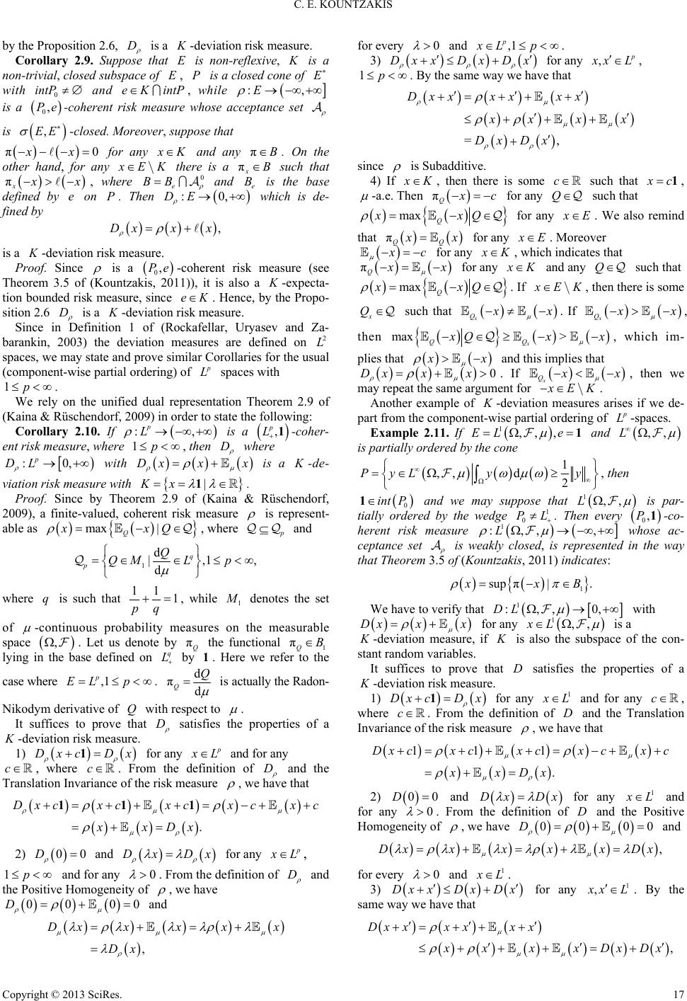 C. E. KOUNTZAKIS by the Proposition 2.6, D is a -deviation risk measure. K Corollary 2.9. Suppose that is non-reflexive, is a non-trivial, closed subspace of K , is a closed cone of PE with and , while 0 intP e KintP :,E is a 0,Pe-coherent risk measure whose acceptance set is , E -closed. Moreover, suppose that π0xx for any K and any π . On the other hand, for any EK there is a πx such that x π x, where 0 e BB and e is the base defined by on . Then which is de- fined by eP ,:0DE x Dx ,x is a -deviation risk measure. K Proof. Since is a 0-coherent risk measure (see Theorem 3.5 of (Kountzakis, 2011)), it is also a -expecta- tion bounded risk measure, since . Hence, by the Propo- sition 2.6 ,Pe eK K D is a -deviation risk measure. K Since in Definition 1 of (Rockafellar, Uryasev and Za- barankin, 2003) the deviation measures are defined on 2 spaces, we may state and prove similar Corollaries for the usual (component-wise partial ordering) of spaces with . 1p We rely on the unified dual representation Theorem 2.9 of (Kaina & Rüschendorf, 2009) in order to state the following: Corollary 2.10. If :, p p L 1 is a -coher- ent risk measure, where , then , p L1 D where :0, p DL with is a Dx x x -de- viation risk measure with |Kx 1. Proof. Since by Theorem 2.9 of (Kaina & Rüschendorf, 2009), a finite-valued, coherent risk measure is represent- able as max |xQ Q x, where and 1 QM d |, 1, d p Qp q L where is such that q11 1 pq , while 1 denotes the set of -continuous probability measures on the measurable space . Let us denote by Q the functional 1Q , π π lying in the base defined on q by 1. Here we refer to the case where . ,1 p EL pdQ πQd is actually the Radon- Nikodym derivative of with respect to Q . It suffices to prove that D satisfies the properties of a -deviation risk measure. K 1) for any Dxc Dx1 L and for any , where . From the definition of ccD and the Translation Invariance of the risk measure , we have that . Dxcxc cxcx xxx 11 1 x D c 2) 00D and Dx Dx for any L , 1p and for any 0 . From the definition of D and the Positive Homogeneity of , we have 00 00D and , Dx xx Dx xx for every 0 and ,1 p xL p . 3) x DxDxxD for any , xL , 1p . By the same way we have that =, Dxx xxxx xx Dx Dx x since is Subadditive. 4) If K , then there is some such that c c 1, -a.e. Then πQ c for any such that Q maxx QQx for any E. We also remind that πQQ x for any E. Moreover c for any K , which indicates that πQ x for any K and any such that Q maxxx Q Q . If EK, then there is some x Q such that x Q x . If x Q x , then > x max QQ Qx x , which im- plies that x and this implies that 0xx Dx . If x Q x , then we may repeat the same argument for EK . Another example of -deviation measures arises if we de- part from the component-wise partial ordering of -spaces. Example 2.11. If 1 EL ,,,e 1 and ,,L is partially ordered by the cone 1 ,,d 2 PyLyy , then 0 int P1 and we may suppose that 1,,L is par- tially ordered by the wedge . Then every 1 0 PL 0-co- herent risk measure ,1P 1 L:,, , whose ac- ceptance set is weakly closed, is represented in the way that Theorem 3.5 of (Kountzakis, 2011) indicates: 1 sup π|. xB We have to verify that 1 :,, 0,DL with Dx xx for any 1,,xL is a -deviation measure, if is also the subspace of the con- stant random variables. It suffices to prove that satisfies the properties of a D -deviation risk measure. 1) Dx cD x1 for any 1 L and for any c , where c . From the definition of and the Translation Invariance of the risk measure D , we have that 11 1 . Dxcxc xcxcx xxDx c 2) 00D and Dx Dx for any 1 L and for any 0 . From the definition of and the Positive Homogeneity of D , we have 0000D and ,Dxx xx xDx for every 0 and 1 L . 3) Dx xDxxD for any 1 , xL . By the same way we have that , Dx xx xx x xxxDxDx Copyright © 2013 SciRes. 17  C. E. KOUNTZAKIS since is Subadditive. 4) x if K, since cc 1, and cc1 c1 if K , which implies that in this case. Also, we may notice that if Dx x x 0 K, then there is a co-set with 0 yK0 yK , such that 0 yK. Then 00 yk 1 for some 0 k . But from the first property , hence it suffices to prove that Dx D 0 y 00Dy in any equivalent case. Notice that if K , then π x for any π . This implies that if , then there is some 0 yK0 π such that 00 0 yy π. If 00 π0 yy , then πy y 0000 sup ππyB , which implies what we wanted to prove. If 00 0 πy yK y, then apply again the previous argument for . 0 Since the value of a risk measure at any financial position has both the financial and the actuarial interpretation of the premium, the term corresponds to a standard term of the risk premium, which is related to the geometry of the ac- ceptance set. When the acceptance set is the positive cone 2 of the space of the square-integrable risks, then this standard term is the mean value , since in this case. The last case is the usual attitude towards risk, under which a non-risky position is a position whose outcomes are positive 1 -almost everywhere in . The subspace mentioned in the Definition 2.3 above, may be considered to be a subspace of non-risky assets. For this reason, the addition of such an asset does not affect the pre- mium calculation, according to the first property of the - deviation measures. However, the whole theory of -devia- tion measures can be developed without reference to the partial ordering. K Consider a proper subspace of assets (which are considered to be the non-risky ones), denoted by . Definition 2.12. A -deviation risk measure :0,DE satisfies the following properties: 1) Dx kDx for any E and for any c , where , where kK is a closed subspace of . E 2) and for for any 00D Dx Dx E and for any 0 . 3) Dx xDxDx for any , xE . 4) for any 0Dx EK , while if Dx0 K. The definition of the -expectation-bounded risk measures is the following: Definition 2.13. A expectation-bounded risk measure :,RE Rx ck satisfies the following properties: 1) for any cRx E and for any , ckK 2) 0=0R and = xRx for any K and for any 0 . 3) x xRxRx for any , xE . 4) xx for any EK, while if Rx x K. Proposition 2.14. A -deviation measure defines a seminorm K D on . Proof. The conclusion is immediate, since by property is positively homogeneous and by property is subadditive, hence it is sublinear, according to Definition 5.32 of (Aliprantis and Border, 1999). This implies by Lemma 5.33 of (Aliprantis and Border, 1999) that the function defined by ( )ii D D( )iii : D gE max , D xDxDx is a seminorm on . Actually, max , D xy Dxy Dxy and since D is Subadditive, we have that yxD y,DxDy DxyDDx . Hence max , max ,max , DD y DxyDx Dx Dx gx gy , D gx y Dy Dy by the properties of maximum of real numbers. Hence is Subadditive. Also, by Homogeneity Property of , we have that D max , max , D xDx Dx D D x x if 0 and also by well-known properties of maximum of real numbers, max ,. DD xDxD xg x If 0 , then max , max , D gx DxD Dx x Dx which is equal to D x for the same reason. Also, if 0 then max0 ,00 DD XDD g x for any E . Finally, DD xg x for any E and any . The same proof may be repeated for -deviation measures defined on partially ordered spaces. Corollary 2.15. A -deviation measure defines a se- minorm D on . Also, by the above Proposition, another Corollary arises for the deviation measures which were initially defined on 2,,L . Corollary 2.16. A deviation measure defines a semi- norm D on 2,,L . Another result concerning seminorms is the following. Proposition 2.17. A seminorm defined on such that p E 0KxEpx is a -deviation measure. K Proof. It suffices to prove that satisfies the properties of a -deviation measure. p K 1) px kpx for any E and for any kK . This holds due to the subadditivity property of the seminorm according to which, p px kpxpk and ,pxpxkpk while 0, 0pkp k for any . Hence the equality ,kKxE px kpx is true. 2) 00p and p xpx for any E and for any 0 , since px px for any and any E . 3) px xpxpx for any , xE , from the subadditivity of the seminorm . Copyright © 2013 SciRes. 18  C. E. KOUNTZAKIS 4) for any 0px EK, while if 0px K. Consider the co-sets . Every ,yKyE E belongs to some of these co-sets. If K, then it belongs to the co-set 0 K, hence px 0 holds. If EK K, then it belongs to some co-set of the form 0, where . Then y 0 yK00 y k p k 0y for some . This implies . 0 kK px py 00 0 Again, by the above Proposition, we obtain another Corol- lary for the deviation measures which were initially defined on 2,,L . Corollary 2.18. A seminorm defined on p such that 0KxEpx xExcc 1,, is actually a K-deviation measure. The same proof may be repeated for -deviation measures defined on partially ordered spaces in the sense we defined them before, hence we obtain the following K Corollary 2.19. A seminorm defined on such that 0,KxEpx xExcec , where eB , is actually a -deviation measure. K Proof. In both of cases of 2 and the case of the above Corollary, we repeat the proof of Proposition 2.17 In the case of 2 we replace by c, while in the case of an or- dered Banach space we replace by , where . kK 1kK,cee B c Example 2.20. Consider a set of continuous linear function- als i iI of , where 1 i in and fEI . Also, suppose that iI kerf ∩, where 0i K. Then the functional , where : I pE sup Ii xfxiI is a seminorm on with E 0 I Ep xK . Note that I px is a real number for any E since sup Ii pxxiI x.f For the subadditivity of p we have that sup sup sup sup , ii ii ii II px yfx yiI fxfyiI xi Ifyi I px py from the well-known properties of the suprema of subsets of real numbers. Also, about the positive homogeneity of p we have that sup sup sup . Ii i iI pxf xiIfxiI fxi Ipx Since iI kerf ∩, then 0 Ii. For the inverse inclusion, suppose that KxEpx 0 I py for some yE . Then sup fyiI0 i. The last equality implies 0sup ii fy fyiI 0, for each i. Then I 0 i fy i for each i, which im- plies that iI I kerf K∩. Then, is actually a -de- viation measure. K Proposition 2.21. If a -deviation measure is of the form K indicated in the Example 2.20, it is Lipschitz-continuous. Proof. According to what is indicated in the Example 2.20 . I px x By subadditivity, , II I px pxy py since xy y . By the same way, , II I pypyxpx since yyxx . By the last two inequalities, ,. III III px pypxypy pxpyx Since II pyxpxy for any , yE, this implies . III x pypxyxy Hence, is a Lipschitz-continuous function. Support Functionals and the Dual Characterization of -Deviation Measures K In this Section we extend the duality characterization Theo- rem Theorem 1 of (Rockafellar, Uryasev, & Zabarankin, 2003) which is proved in the case where the space of financial posi- tions is 2 in the case of -deviation measures being de- fined on Banach spaces. K Theorem 3.1. A functional :0,DE is a lower semicontinuous K-deviation measure if and only if it has a rep- resentation of the form infsup , fF fF Dx xfx xfx where FE is non-empty, weak-star closed and convex, E is a linear functional which corresponds to a “standard premium term” for any E , 0K and D xF kerx ∩, where ,FxExffF D. Also, if we suppose that E is partially ordered by the cone , where is a wedge of 0 PP , then for any EK there is some x F such that x fx if 0D P. Under this dual represen- tation, F is determined by ,.FfEDx xfxxE Also, if is finite-valued then this is equivalent to the fact that D is bounded. Proof. Since is a lower semicontinuous -deviation measure, by Theorem 5.104 of (Aliprantis & Border, 1999) is the support functional of the weak-star closed, convex subset of DK D * E ,. D FxExxDxxE The last Theorem implies that supDxx x D xF for any E . Since 0Dx for any K, the last dual representation implies 0xx for any F . This indi- cates , kerx x F. Hence D xF kerx ∩. But also for the inverse inclusion, we get that if D xF kerx ∩ then 0Dx , which means that if K, then 0Dx . We have that 0 D xF kerx ∩ because we suppose that 0K . If we suppose that the functional provides a standard “premium term”, we define E , FfExfxF . Then Copyright © 2013 SciRes. 19  C. E. KOUNTZAKIS , FfEf xxF F is also a weak-star closed, convex subset of E . Then in terms of we also take the following dual representation: supinf . fF fF Dxxfxxfx If F is a bounded set then is a bounded set and this implies that is finite-valued, because F D sup sup DD xF xF DxxxxxMx o , where 0M is an upper bound for the norms of the elementsf F. Converselyf D is finite-valued, then sin, ice xDx for any E, where F , we get xDx and finally max , xDxDx . For any F we have supmax,. D xF xxDxDx Hence sup D xF from the Uniform Boundedness Principle and this implies that x is bounded. This is actually a characterization of -deviation risk measures defined on a Banach space . For the inverse direc- tion of the proof, suppose that the functional :0,DE with infsup, , fF fF Dx xfxxfxxE where E is non-empty, weak-star closed. Then is a lower semicontinuous D -deviation measure, where D xF kerx ∩ with 0K and ,f Dx FxE fF. Let us verify the properties of these risk measures: 1) supsup D Dxkxxkx xDx 0xk D xF kkerx ∩ D xF xF , since for any . 2) sup sup sup D DD xF xF xF Dx xxx x xxxDxD x from the properties of supremum. 3) sup sup DD xF xF Dxx xxxDx 0 for any . Also, 0=0D is obvious. 4) for any 0Dx K, and this holds from the defi- nition of . On the other hand if EK then there is some 0 F such that 00xx . If , then we have that xx 00 0 xxxx sup D xF x 0D. If K is such that , then since also 00xx E Dx xx K 0 xx sup D xF we have and . 0 0 xx 0 Also, is a lower semicontinuous function defined on because it is the supremum of a family of lower semicontinuous functions on . The family is the set of linear functionals D E E F . The Min-Max Approach on the Risk Minimization for Deviation Risk Measures in L2 In this section we consider the following risk-minimization portfolio-payoff selection problem: Minimizesubjectto,xx (1) where is a risk measure (not necessarily coherent) and is a portfolio-payoff selection set. The subject of this section is to investigate the saddle-value form of the solution for the problem 1, if is some deviation measure in the sense defined in (Rockafellar, Uryasev and Za- barankin, 2003). It is well-known that the portfolio selection problem 1 is a part of the efficient portfolio selection theory and practice, see (Markowiz, 1952), (Kroll, Levy, & Markowitz, 1984). We remind that the classic form of a zero-sum game between two players has as payoff function the bilinear form of a dual pair , X and the strategy set of the one player may be id- entified by a set , while the strategy set of the other player may be identified by some . The payoff , x is understood to be a reward paid from the first player to the second. By selecting x , the first players’ maximum loss is max , x x . By choosing a proper strategy , he may 0 x achieve to pay to the second player no more than the minimum of these losses, which is equal to 0min max, xx x , if this quantity is well-defined. On the other hand, for any str- ategy of the second player the minimum payoff he earns is x min , x x and by choosing a proper strategy x , he may achieve to receive from the first player at least the maximum of these earnings, which is equal to 0max min, x x x , if this quantity is well-defined. 0 000 ,xx holds and if the equality holds, then the common value is called saddle-value, while the pair 00 ,xx which is the solution point of the game, is called saddle-point. We may replace the bilinear form , by another payoff function defined on and the no- tions are repeated in the same form. For a brief explanation on zero-sum games which leads to the min-max theorems, see in (Luenberger, 1969). Also, a primal reference for zero-sum games is (von Neumann, 1928). The saddle value sup inf xy v, sup,F xyFF xy inf ,xy y x , can be interpreted as the value of a zero sum game between two players. The one player minimizes ,Fxy over suppos- ing that the other player follows the strategy , while the other player maximizes ,y y Fx over supposing that the other player follows the strategy , see also (Kountzakis, 2011). We remind the statement of Corollary 3.7 of (Barbu & Pre- cupanu, 1986) in Paragraph 3.3 of (Barbu & Precupanu, 1986): If , Y are reflexive Banach spaces, , Y are bounded, closed and convex sets, is an upper-lower semi- continuous, concave-convex function on , then has a saddle point on , namely a pair ,xy such that supinf,inf sup,,. yy xx xyF xyF xy Also, we give the following definitions of the payoff func- tions: Definition 4.1. A function :F is concave- convex like if the following conditions hold: 1) for every 12 ,xx and 0,1t there is a 3 x such that 12 ,1 ,,tF xytF xyFxy 3 Copyright © 2013 SciRes. 20  C. E. KOUNTZAKIS for all . y 2) for every and 12 ,yy 0,1t there is a 3 y such that 31 ,,1Fxy tFxytFxy 2 , for all . x Definition 4.2. A function :F is quasi-con- caveconvex if the level sets 0 |, Fxy a and 0,yFxya are convex sets for every and . 00 ,xy a Definition 4.3. A function :F is called con- cave-convex if it is concave in the first variable and convex in the second variable. We remark (see also Remark 3.5 in (Barbu & Precupanu, 1986)), that a concave-convex function is both concave-con- vex-like and quasi-concave-convex. According to Theorem 3 in (Rockafellar, Uryasev, & Za- barankin, 2003), by considering some set of elements con- sisted by random variables such that 2 QL d 1Q , or else density functions ( d d Q Q , where Q denotes the corresponding probability measure), the risk measure 2 :0,DL with inf |EXQQ DX EX is a deviation risk measure. is a subset of the base of 2 2 defined by the constant random variable which is a strictly positive functional of it. The set as it is mentioned in p. 17 of (Rockafellar, Uryasev and Zabarankin, 2003) is considered to be a convex and closed of the base defined by on 1 . This base is un- bounded because 2 induces a lattice ordering on 2 . The dual form infDX EXEXQQ of a deviation measure if is convex, closed and bou- nded and we consider some financial positions’ choice set for an investor denoted by , which has the same properties and it is a subset of D 2 , drives us wonder whether Corollary 3.7 of (Barbu & Precupanu, 1986) and its game-theoretic implication can be applied in the case of the risk minimization problem. The boundedness of in this case simplifies the saddle- value solution of the problem. Actually, we suppose that we have the following version of the risk minimization problem 1: Minimizesubject toDX X (2) Apart from the Proposition 2 in (Rockafellar, Uryasev, & Zabarankin, 2003) which indicates that finite-valued deviation measures on 2 being lower semicontinuous are norm-con- tinuous, we prove a stronger result than Proposition 2 in (Rockafellar, Uryasev, & Zabarankin, 2003), since it indicates that they are Lipschitz continuous in the case we consider. Proposition 4.4. Any deviation measure 2 :0,DL 2 , where is a convex and bounded subset of such that 1EQ Proof. We have to prove that is a norm-continuous function on is a Lipschitz function. D 2 . But if is a norm-bounded set, this implies that is a Lipschitz function. This is true because for two families of functions such that ,: ii fg D 2 L sup ,sup ,sup iii i fX gYiIfXiI gYi I and for any 2 , YL that satisfy the above finite suprema conditions, supsup sup ii ii XgYiIfXiI gYiI is true. Hence if I , 1 QQ XgXEX Q and since XY Y 2 , for any YL, this implies sup 1 sup 1 sup 1 . DXEX QQ EXY QQ EY QQ DXYDY By the same way we have that ,DYDY XDX since YYXX . Finally, 1 1DXXY QDY E , where 1 Q be- cause since is convex, closed and bounded subset of a reflexive space, it is a weakly compact subset of it and the su- premum in DXY Q is actually a maximum. Hence we consider 1 to be a maximizer of Y over . In the same way, XE Y 2 Q 1X 2 Q DYD , for some . Hence, 22 2 2 111 1, EXYQXYQ XYQ XY m 2 for some upper bound of the norms of the elements of . Proposition 4.5. If we suppose that and are convex, closed and bounded, the problem 2 has a solution. Proof. Since is a norm-continuous function, then the problem 2 has a solution, since is also weakly lower semi- continuous and is a weakly compact set. D D Since the problem 2 has a solution, it has an optimal value. We will investigate whether this optimal value is a saddle value, according to Corollary 3.7 of (Barbu & Precupanu, 1986). The duality form of , implies that the candidate two- variable function for the application of Corollary 3.7 of (Barbu & Precupanu, 1986) is D :F , where ,1,,FQXE XQQX . For this function we have the following. Proposition 4.6. The function satisfies the properties of Corollary 3.7 of (Barbu & Precupanu, 1986), hence the optimal value of the risk minimization problem 2 is a value of the function :F , namely 00 inf, ,DXX FQX for some 00 ,XQ . Proof. is upper-lower semicontinuous, because it is norm-continuous in both of its variables. Moreover, it is linear in both of its variables, which implies that it is concave-convex. Hence the conclusion is true from Corollary 3.7 of (Barbu & Precupanu, 1986). The economic interpretation of the fact that the risk minimi- zation problem is solved through determining a saddle-point of the function is the following: The minimization of risk corresponds to a zero-sum game between the investor and the market. The payoff function of the game—the one which is Copyright © 2013 SciRes. 21  C. E. KOUNTZAKIS minimized by the investor as a cost function for a given “valua- tion” density over the set of financial positions is the partial function . The function being maximized as a “value” function for a specific financial position Q ,FQ by the market over the set of valuation densities is the partial function ,X F. The value of the game, which is also the optimal value of the risk minimization problem 2 is achieved at a saddle point 00 ,QX. This meets the notion of a “two-per- son zero-sum game” for one more reason, because the market can be viewed as a whole to which the monetary cost of the risk minimization is paid (the one player) and the investor can be viewed as the other player who earns the monetary payoff con- cerning a certain financial position , which is formulated by the market as the value of it. To be more accurate, suppose that the set of strategies of the market is the set of the valuation measures , while the set of strategies of the investor is the set of the financial positions . If we select some X , the investor’s maximum loss is maxQ,FQ X . By choosing a proper strategy 1, she may achieve to pay to the sec- ond player (to the market) no more than the minimum of the above costs, being X 1 mi n max,FQ XQ, if this quan- tity is well-defined. On the other hand, the market for any strategy of it, the minimum payoff that it earns from the investor is X Q min ,X X and by choosing a proper strategy 1, it may achieve to receive from the investor at least the maximum of these earnings which is FQ Q 1, if this quantity is well-defined. If there is a max min QX ,FQ X 00 ,QX such that 0 Q 1 10 X , then 0 is a solution to the deviation minimization problem 2. For a similar explanation on saddle-value form that minimiza- tion of convex risk measures may take, see also in (Kountzakis, 2011). The Risk Minimization for Deviation Measures on Reflexive Spaces: Bounded Sets In this section we prove the existence of solution to the problem of minimization of deviation if the deviation measure comes from a certain class of coherent risk measures. Specifically, if we transfer the above results to the frame of the commodity-price duality ,EE , where the space denotes a reflexive space in which the financial positions lie in, then we get a saddle-point solution result for the following minimization problem ,subject t Pe Dx ntP E Minimi , zeo , E x ei P (3) where is a convex, closed, bounded subset of , is closed and and , and Pe denotes a intP ,E : ,Pe -coherent risk measure on . The closed subspace E is such that for any K , π, xxK holds for any π , while for any EK, there is a πx such that πx x. Also 0 , e e BB . The functional is de- fined as follows: ,: Pe DE ,0 ,x ,Pe 0 sup ππx BDx where e B and e is the base defined by on . e 0 P , 0 e , is the dual wedge of e Theorem 4.7. The problem 3 has a solution via saddle- points. in . E Proof. According to the above dual representation for , e D , we get that ,supππ,. Pe Dxxx Bx In order to apply Corollary 3.7 of (Barbu & Precupanu, 1986) in this case, we have to determine the payoff function :F , where , Y are convex, closed and bounded subsets of the reflexive spaces , Y ,B and has to be a concave-convex and upper-lower semicontinuous function. We notice that F ,,XE YE and :FB with π,πFx x x. is concave- convex and upper-lower semicontinuous. Then a saddle-point 00 π,xB exists, or else , 00 π,supinfπ,infsupπ,inf Pe xx x BB . xFxFxD x According to the saddle-point conditions for 00 π, , , 00 0 π,Pe FxD x . The Minimization of Deviation Measures in Banach Spaces: Unbounded Sets The question which arises is whether the above min-max ap- proach for the minimization of deviation measures can be gen- eralized in the case of an unbounded choice set of financial (risk) positions. The answer is affirmative due to an alternative min-max theorem reminded in p. 10 of (Delbaen, 2002). We also focus on the classes of deviation measures related to the coherent measures arising from ordering cones with non-empty interior. Specifically, the statement of the previously mentioned min-max theorem is the following: Let be a compact, con- vex subset of a locally convex space . Let Y be a convex subset of an arbitrary vector space . Suppose that is a bilinear function u :uX Y . For each , we suppose that the partial (linear) function lL ,ul is continuous on Y. Then we have that inf sup,supinf,. lL lL kK kK ulk ulk Then we have the following Theorem 5.1. Suppose that is a reflexive space. Con- sider the problem E , Minimizesubjectto, Pe Dx x (4) where is a convex, unbounded subset of , is closed and P intP , and eintP , . The closed subspace is such that for any E K K , π, xxK holds for any π , while for any EKπ, there is a xe such that x x . The functional ,Pe :DE0, is defined as follows: ,sup , Pe Dxx B x where ,Pe e 0 B and e is the base defined by on . Then the problem 4 has a solution. e 0 PProof. If we apply the previous min-max theorem, we have that YE endowed with the weak topology, E , ,KBL . is a locally convex space, Y is a linear space, , :uE E ,,x,uxx x E E . The functional E x is the one specified by assumptions. Also, for any , the partial function Copyright © 2013 SciRes. 22  C. E. KOUNTZAKIS ,: x uxu E where x ux x for any E and hence for weakly any xon x u is continuous, since if we sider a net . The partial functi con aaAE such that ,EE a , for the specific E, a x , then w et e g ,,xx . aa ux x xa x uu xux Finally, for each E and for eac y parti h specific es that anal function , x ux E x. This impli is continuous, which is also valid for any xso, u is a bilinear function as it arises from its defi. Since base e weakly the niti on . Al of the cone P is convex and weakly compact, the set i sio s weakly compt and convex, too. Also, the set is convex and the conditions for the validity of the conclu- n of the previous min-max theorem hold. Hence the min- max equation holds for u, which implies the existence of a saddle-point ac 11 , B such that infp ,suDx ux ,Pe ,1 pinf , ,. Pe x BB ux D x 11 sui nf xx ux int is implied by Pro eorem for non-re t le-po position flex The existence of a of prove na .2. S sadd 3.1 the corresponding Th uppose tha (Barbu & Precupanu, 1986) which says that a function satisfies the min-max equality if and only if it has a saddle- point. We ive Ba- ch spaces. Theorem 5 is a non-reflexive Bana ch space. Consider the problem ,subjectto, Pe x x nvex, unbounded subset of 0 MinimizeD (5) where is a co . If P is a closed cone of E and 0 intP and 0 eitP, E n and 0,:, Pe E denotes a Prent ris meas ure on 0,e-cohe k . The closed subspace Kch that for any is su K, , xxK holds any e for , while for any EK, there is a xe such that x x . Then the al function , 0 Pe :DE 0,, where ,x , 0 Pe Dx is a 1 sup x B -deviation risk mhere easure, w0 e 1 B and e ais the base defined by e on P. Then 5 has solution. Proof. I the problem x theorem,f we apply tha the previous min-mae we hav t YE endowed with the weak-star topology, E , K. Y is a locally convex space, E is ar E, 1,BL space, :uE linea ,,,uxxxE E x . The funis is a linear spaceE , ctional E , :uE tcified bhe one spey assumptions. E ,ux xE ,E, x x . Also, for any x , the partial function ,: xE ux u where x ux x for any E and hence nction x ueak-star continuous, si a net for any x. The partial fu if we consider is wnce aaA E such that ,EE a , for the specific E, a x , then w e get , a uxxxx x . Fi,na a uxlly, xa x uu for each E any p and for each specific plies that artial function , x ux E x. This im is weak-star continuous, which is also valid for any x . Also, u is a bilinear function as it arises from its defi Also, ce the base e nition. sin is weak-star compact and convex base of the cone P, thethe set 1 n is a weak-star compact and con- vex subset of E and the set is a convex subset of , then the condits for the valiy of the conclusion of previous min-max theorem hold. Hence the min-max equation holds for u, which implies the existence of a saddle-point ion ditthe 22 1 , B such that inf sux 11 , 0 222 supinf, ,. Pe xx x BB ux D x ,ux , 0 Pe inf p ux D le-po nt isThe existence of a saddi implied by Proposition 3.1 at of we (Barbu & Precupanu, 1986) which says that a function satis- fies the min-max equality if and only if it has a saddle-point. Remark 5.3. We remind for the sake of completeness of wh proved in the last two Theorems that the fact that if eintP then 0 P has a ,EE -compact base is men- Propoon 13.8.1 eson, 1970). The weak- star compactness of bases defined by elements of tioned insiti2 in (Jam on cones of E is implied in non-reflexive spaces from theroposition Proposition 2.4 of (Kountzakis, 2011), which is actually a reference to Theorem 39 of (Xanthos, 2009). p Minimization ofDeviation Measure the Usual Arising from a S is identicaExpected shortfall a ES che, l to a CVaR . CVaR sche, as Corollary 4.3 in (Acerbi & Tas 2002) indicatesa is initially defined in Definition 2.5 of (Acerbi & Ta002), while a ES is a coherent risk measure on 2 1,,L (see Proposi- 3.1 in (Acerbi & Tasche, 2002))ted in (Acerbi & Tasche, 2002), the expression tion . As it is quo 0 1d a ESxq xu au a block for law invariant, indicates that a ES easu is the building coherent risk mres, according to the results containing in (Kusuoka, 2001). These properties of a CVaR may make it very attractive in applications, since it replace a VaR . Also, as it is mentioned in (Rockafellar, Uryasev, & Zabar 2003), a shortfall relative to expectation is more adequate in practice. A very interesting application of the saddle-point method in order to verify the existence of solution to the minimization of deviation risk is also by the use of min-max Theorem mentioned in p. 10 of (Delbaen, 2002) in the case of the “deviation which arises from expeced shortfall”, which is defined as the functional could ankin, 1 :,, 0,DL with 1 , aa Dx ESxxxL ,, f sig- level for a o nificance 0,1 .a As it is well-known from Acerbi and Tasche, 2002) and (Tasche, 2002) the expected shortfall a ESx for a financial position and a level of significance 0,1 is defined in Definition 2.6 of (Acerbi & Tasche, 2002) as the negative of tail-mean of a at the level a, being equal to 1,xxaxqx 1a xq x aa qa ES ere x E a wh a qx denotes er quantile of the a-low . T Z he deviatio sure D is introduced in Example 4 of (Rock- afellar, Uryasev, &abarankin, 2003). Also, expected shor- n mea Copyright © 2013 SciRes. 23  C. E. KOUNTZAKIS tfall according to Theorem 4.1 of (Kaina & Rüschendorf, 2009) admits the dual representation mESx ax , a aQ Qx where 1 d1 ,-a.e. d a Q QM a . 1 denotes the set of -continuous probability measures on the measurable space ,. 1 d,, QL d esentation set . But for the probability measures of the repra , d1 0, d Q a 1 holds, with res- the usual (point partial ordering on pect towise) ,,L . This implies dQ,, dL for any Lemma 5.4. a Q. d d a QQ a is a weak-star compact set of ,,L . We coider the set Proof. ns d 1, ,, d aa Q Qca QQ and is the order-interval a 1 0, aa 1 of which is 1 , L Border, 19 -compact due to Lemma 7.54 of (Aliprantis & 99). We also have to prove that a is weak-star closed in . Let us consider a net a QZ such that 1 , dLL Q. d From the fact that d, d Q , we obtain that 1 d,, d QL . We have to prove that is a Radon- Nikodym derivative of some measure with respect to 1a Q . Let us consider the map 1:Qere 0,1 wh 1d A QA fI and I is the characteristic random variable of . In order to show that 1 Q is a probability measure, d,Qf 1 which is the limit limdQ and every of the terms of the net of real numbers d,Q is equal to . By the same argument, we may deduce that Hence, where denotes the set of natural numbers. For from the 1 en 10Q . If nn A is a sequence of sets in which are disjoint, th 1 1 ,. n n kk k k QA QA ∪ 11 1 1 ,, n n kk k k QA QAn ∪ n 11 1 1 , nnn n QA QA ∪ 1 , L -convergence 1 , d, LL Q d and the definition of , the fact that ay characteristic func- tion 1 Qn , A IA belongs to 1,,L . We may also refer to the Monotone Convergence Theorem (11.17 in (Aliprantis & Border, 1999), where the restriction of the f on the set 1nn ∪ is the integrable function which is mentioned in the Theorem, while n is the restriction of f on a set of the form n 1kk ∪. For the -continuity of 1 Q, we have that if for a set A 0A holds, then since ,Q is -conti- nuous, d 0 Q QA d , d A for any . But since 1 , d, LL Q d then 1 d dlim d0 d AA Q QA f . Hence is 1 Q -continuous. Since are prob- ability mes, ,Q easur d0, Q d -a.e. Also, since is a 1 Q -continuous probability mea- y Radon-Nikod Th we have sure, bymeorem 1 d, d Q -a.e. and 0f , -a.e. In order to show that 1 0,fa 1 with respect to the usual (point-wise) partial ordering on ,,L , we use the convergenceent argum ddd, d AA Q for any A . This implies that 1 d0f, Aa for any A . Tplies his im1 0fa 1 -ae suppose does not hold some B .e., since if w , then th existsthat thisere with 0B such that either 1 fa, or 0f for any . Then, we would have either 1 df d 0 Bf B a, or , adiction. Finally, the set eak- of a weak-star compact set whet a contr is a wstar closed subset is the s The above deviation measure is denoted b a ich a. y a Da CVaR in Copyright © 2013 SciRes. 24  C. E. KOUNTZAKIS (Rockafellar, Uryasev, & Zabarankin, 2003), see p. 7 in (Rock- afellar, Uryasev, & Zabarankin, 2003). Hence, we have the following risk minimization problem Minimizesubject to a CVaR xx (6) The existence of solution to the risk minimization problem 6 does not depend on the fact whether the set positions which is the selection set of the investor is bo of financial unded or not. Theorem 5.5. If is a convex set of 1,,L , then the deviation risk minimization problem 6 has a solution. Proof. We will apply the min-max theorem reminded in p. 10 of ndowed w (Delbaen, 2002). We have that YL eith the weak-star topology, 1 L, ,KL a . Y is a locally convex space, 1 L is a linear space, 1 :uLL 1 ,,,uxxx xL e notice that u is a bilinear function ova defined and this arises by iinition. The partia L . W duct of the l f er the pro ef sp un ces ction ts d ,xu is actually the function :uL xre x uxxxx 1. This function is weak- star continuous for any 1 , whe L and consequently for a x. By 1 we random variab is a net in ny le for which denote th . Suppose that e 1, 1 , which is 1 , L -converge some nt to . Hence for any 1 L and of course for any specific x, x . Also, x and fin ally ,uxx xux ,x x . But is specified, hence xx uu funct subset of h weak-s the partial w io ich n implie : x uL 1 s t he . tar Hence since continuity of is a convex and a is a ak-star compact, convex s weubset of , all the conditions of the min-max Theorem reminded in p.10 of (Delba valid. Hence thin-max equation holds for , whicplies the existence of a saddle-point en, 200 uh i 2) a m re e m ,a Q x such that infinfsup,sup, Qa aQQ xx CVaRxuxu x ,. Qa x a Q ux CVaR x inf The existence of a saddle-point is implied Proposition 3.1 of (Barbu & Precupanu, 1986) which says that a function satisfies the min-max equality if and only if it has a saddle-point. Acerbi, C., & Tasche, D. (2002). On the coherence of the expected shortfall. Journal of B1487-1503. doi:10.1016/S0378-4 REFERENCES anking and Finance, 26, 266(02)00283-2 Aliprantis, C. D., & Border, K. C. (1999). Infinite dimensional analysis, A hitchhiker’s guide (2nd ed.). New York: Springer. doi:10.1007/978-3-662-03961-8 Artzner, P., Delbaen, F., Eber, J. M., & Heath, D. (1999). Coherent measures of risk. Mathematical Finance, 9, 203-228. doi:10.1111/1467-9965.00068 Barbu, V., & Precupanu, T. (1986). Convexity and optimization in banach spaces. D. Riedel Publishing Company, Kluwer Academic Publishers Group, Dordrecht. Delbaen, F. (2002). Coherent risk measures on general probability spaces. In: Advances in finance and stochastics: essays in honour of Dieter Sondermann (pp. 1-38). Springer-Verlag: Berlin. doi:10.1007/978-3-662-04790-3_1 Denis, L., & Martini, C. (2006). A theoretical framework for the pricing of contingent claims in the presence of model uncertainty. Annals of Applied Probability, 16, 827-852. doi:10.1214/105051606000000169 Dhaene, G., Goovaerts, M. J., Kaas, R., Tang, Q., Vanduffel, S., & Vyncke, D. (2003). Solvency capital, risk measures and comonoto- nicity: A review. Research Report versity of Leuven. OR0416, Leuven: Catholic Uni- Gong, X. H. (1994). Connectedness of efficient solution sets for set- valued maps in normed spaces. Journal of Optimization Theory and Applications, 83, 83-96. doi:10.1007/BF02191763 echuk, B., MolybohGra, A., & Zabarankin, M. (2009). Maximum en- tropy principle with general deviation measures. Mathematics of Op- erations Research, 34, 445-467. doi:10.1287/moor.1090.0377 echuk, B., Molyboha, A., & Zabarankin, M. (20Gr11). Cooperative Ja emat- Ja inance and Stochastics, 5, 181-200. games with general deviation measures. Mathematical Finance, Forthcoming. meson, G. (1970). Ordered linear spaces. Lecture notes in math ics (Vol. 141). Berlin: Springer-Verlag. schke, S., & Küchler, U. (2001). Coherent risk measures and good- deal bounds. F doi:10.1007/PL00013530 aina, M., & Rüschendorf, L. (2009). OKn convex risk measures on p -spaces. Mathematical Methods of Operations Research, 69, 475- 495. doi:10.1007/s00186-008-0248-3 onstantinides, D. G., & KKountzakis, C. (2011). Risk measures in ordered normed linear spaces with non-empty cone-interior. Insur- ce: Mathematics and Economics, 48, 111-122. an doi:10.1016/j.insmatheco.2010.10.003 Kountzakis, C. E. (2011). On efficient portfolio selection using convex risk measures. Mathematics and Financi al Economics, 4, 223-252. doi:10.1007/s11579-011-0043-4 ountzakis, C. E. (2011). Risk measurKes on ordered non-reflexive banach spaces. Journal of Mathematical Analysis and Applications, 373, 548-562. doi:10.1016/j.jmaa.2010.08.013 oll, Y., Levy, H., & Markowitz, H.Kr M. (1984). Mean-variance versus direct utility maximization. Journal of Finance, 39, 47-61. doi:10.1111/j.1540-6261.1984.tb03859.x usuoka, S. (2001). On law invariant coherent rKisk measures. In: Ad- vances in mathematical economics (Vol. 3, pp. 83-95). Tokyo: Springer. doi:10.1007/978-4-431-67891-5_4 uenberger, D. G. (1969). Optimization by vLector space methods. New M stochastic analysis and applications, Ralized York: John Wiley and Sons Inc. arkowitz, H. (1952). Portfolio selection. Journal of Finance, 7, 77- 91. Peng, S. (2007). G-expectation, G-brownian motion and related sto- chastic calulus of Itˆ o Type. In: abel symposium (Vol. 2, pp. 541-567). Berlin: Springer. Rockafellar, R. T., Uryasev, S., & Zabarankin, M. (2003). Deviation measures in risk analysis and optimization. Research Report 2002-7, University of Florida. ockafellar, R. T., Uryasev, S., & Zabarankin, M. (2006a). Gener deviations in risk analysis. Finance a nd S to chastics, 10, 51-74. doi:10.1007/s00780-005-0165-8 ockafellar, R. T., UryaRsev, S., & Zabarankin, M. (2006b). Master 4 funds in portfolio analysis with general deviation measures. Journal of Banking and Finance, 30, 743-778. doi:10.1016/j.jbankfin.2005.04.00 . Rockafellar, R. T., Uryasev, S., & Zabarankin, M. (2006c). Optimality conditions in portfolio analysis with general deviation measures. Ma- thematical Programming, 108, 515-540 doi:10.1007/s10107-006-0721-9 Rockafellar, R. T., Uryasev, S., & Zabarankin, M. (2007). Equilibrium with investors with a diversity of deviation measures Journal of Banking and Finance, 31, 3251-3268. doi:10.1016/j.jbankfin.2007.04.002 /j.spa.2010.10.006 Soner, H. M., Touzi, N., & Zhang, J. (2011). A martingale representa- tion theorem for the G-expectation. Stochastic Processes and their Applications, 121, 265-287. doi:10.1016 Tand beyond. Journal of Banking asche, D. (2002). Expected shortfall and Finance, 26, 1519-1533. doi:10.1016/S0378-4266(02)00272-8 Copyright © 2013 SciRes. 25  C. E. KOUNTZAKIS Copyright © 2013 SciRes. 26 Von Neumann, J. (1928). Zur theorie der gesellschaftsspiele. Mathema- tische Annalen, 100, 295-320. doi:10.1007/BF01448847 Xanthos, F. (2009). Conic characterizations of reflexive banach spaces. Master’s Degree Dissertation, Athens: National Technical University of Athens.  C. E. KOUNTZAKIS Appendix In this paragraph, we give some essential notions and results from the theory of partially ordered linear spaces which are used in the previous sections of this article. Let be a (normed) linear space. A set satisfying and E CE CC CCC for any is called wedge. A wedge for which 0CC is called cone. A pair ,E where is a linear space and is a binary relation on satisfying the following properties: 1) x for any E (reflexive). 2) If y and then yz z, where , , yz E (transitive). 3) If y then y for any and zyz for any , where zE, yE (compatible with the linear structure of ), is called partially ordered linear space. The binary relation in this case is a partial ordering on . The set E |0Px x E is called (positive) wedge of the partial ordering of . Given a wedge in C , the binary relation defined as follows: C , C yxyC is a partial ordering on , called partial ordering induced by on . If the partial ordering of the space is anti- symmetric, namely if E CEE y and implies yx= y, where , yE, then is a cone. P E denotes the linear space of all linear functionals of , while is the norm dual of , in case where is a normed linear space. E EEE Suppose that is a wedge of . A functional CE E is called positive functional of if for any C 0fx C . E is a strictly positive functional of if for any C 0fx 0xC. A linear functional E 0 where is a normed linear space, is called uniformly monotonic functional of if there is some real number such that E C a xax for any C C. In case where a uniformly monotonic functional of exists, is a cone. C 0* 0fEx xor anyCf Ef CC is the dual wedge of in . Also, by we denote the subset of C 00 0 0 C E . It can be easily proved that if is a closed wedge of a reflexive space, then . If is a wedge of , then the set C 00 CCC E 0 is the dual wedge of in , where denotes the natural embedding map from ˆ Ex ˆ 0f EE or any Cx Ef : fC C to the second dual space of . Note that if for two wedges EE , C of E C holds, then . 00 CKCIf is a cone, then a set is called base of if for any CBC 0xC there exists a unique 0 such that B . The set |Cf 1 f where Bx x is a strictly positive functional of is the base of defined by CC . is bounded if and only if is uniformly monotonic. If is a bounded base of such that C0B then C is called well-based. If is well-based, then a bounded base of defined by a C C EEC exists. If then the wedge is called generating, while if C CECC 0 C it is called almost generating. If is generating, then is a cone of C E in case where is a normed linear space. Also, E is a uniformly monotonic functional of if and only if C 0 intC E , where denotes the norm-interior of . If is partially ordered by , then any set of the form 0 tCin 0 C C ,CC yrEyrx where , yC is called order- interval of . If is partially ordered by and for some C eE , 1n holds, then is called order-unit of . If is a normed linear space then if every interior point of C is an order-unit of . If is moreover a Banach space and is closed, then every order-unit of is an interior point of . ,Ene ∪ E C C nee EE EE The partially ordered vector space is a vector lattice if for any , yE , the supremum and the infimum of , y with respect to the partial ordering defined by exist in P . In this case sup , y and inf , y are denoted by y, y respectively. If so, sup , xx is the absolute value of and if is also a normed space such that x for any E , then is called normed lattice. Finally, we remind that the usual partial ordering of an ,, p L space, where ,, is a probability space is the following: y if and only if the set :xy is a set lying in of -probability . 1 All the previously mentioned notions and related proposi- tions concerning partially ordered linear spaces are contained in (Jameson, 1970). A topological linear space is is boundedly order complete if for every bounded increasing net in the space E E , the supremum of the elements of it exists. A cone of a linear topological space P is called Daniell cone if every increasing net of which is upper bounded converges to its supremum. Note that every well-based cone in a Banach space which has a base defined by a continuous linear functional. Every closed, well-based cone in a Banach space is a Daniell cone. Every Banach space partially ordered by a closed, well-based cone is a boundedly order-complete space. A subset of a convex set in C is called extreme set or else face of , if whenever C 1 az ayF, where 01a and ,yz C implies . If is a singleton, is called extreme point of . ,yz FF FC A family of cones in normed linear spaces having non-empty cone-interior are the Bishop-Phelps cones, also mentioned in (Konstantinides & Kountzakis, 2011). The family of these cones in a normed linear space is the following: E ,L,,,0,1.Kfxfx axfa 1af L A proof for the existence of interior points in these cones is contained in p. 127 of (Jameson, 1970). Another family of cones with non-empty interior is the family of Henig Dilating cones. These cones are defined as follows: Consider a closed, well-based cone in the normed linear space C , which has a base , such that 00,1BB . Let 0,1 be such that 20,1BB , where 0,1B denotes the closed unit ball in . If E 0,1Bc , n K one , n KB n n , then , n1nn CK is a cone for any , 2n 0, n ntn1CiK. About these cones, see for example see Lemma 2.1 in (Gong, 1994). For example, a Bishop-Phelps cone ,faCK in a reflexive space which is a well-based cone as the construction of the n requires, provides a set of interior points ,Kn 0C of the cone . If we , n Kn1 Copyright © 2013 SciRes. 27  C. E. KOUNTZAKIS Copyright © 2013 SciRes. 28 consider the base | f BxCfx 1 defined by , this base is a closed set where 0 . Hence there is a 0, gE such that 0gy for any yB . can be selected to be such that 1g, hence 0ygy . By setting 2 , n Kn , we may construct a sequence of approximating cones , since we can set f , 0,1a . We remind that if is a convex set, then the set D cone| ,DxExdd ,D is a cone D wedge and by we denote its norm (or weak) closure.
|