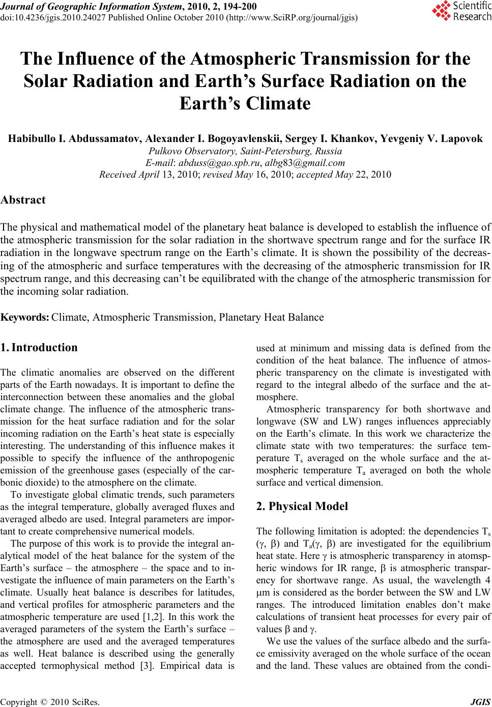Journal of Geographic Information System, 2010, 2, 194-200
doi:10.4236/jgis.2010.24027 Published Online October 2010 (http://www.SciRP.org/journal/jgis)
The Influence of the Atmospheric Transmission for the
Solar Radiation and Earth’s Surface Radiation on the
Earth’s Climate
Habibullo I. Abdussamatov, Alexander I. Bogoyavlenskii, Sergey I. Khankov, Yevgeniy V. Lapovok
Pulkovo Observatory, Saint-Petersburg, Russia
Received April 13, 2010; revised May 16, 2010; accepted May 22, 2010
Abstract
The physical and mathematical model of the planetary heat balance is developed to establish the influence of
the atmospheric transmission for the solar radiation in the shortwave spectrum range and for the surface IR
radiation in the longwave spectrum range on the Earth’s climate. It is shown the possibility of the decreas-
ing of the atmospheric and surface temperatures with the decreasing of the atmospheric transmission for IR
spectrum range, and this decreasing can’t be equilibrated with the change of the atmospheric transmission for
the incoming solar radiation.
Keywords: Climate, Atmospheric Transmission, Planetary Heat Balance
1. Introduction
The climatic anomalies are observed on the different
parts of the Earth nowadays. It is important to define the
interconnection between these anomalies and the global
climate change. The influence of the atmospheric trans-
mission for the heat surface radiation and for the solar
incoming radiation on the Earth’s heat state is especially
interesting. The understanding of this influence makes it
possible to specify the influence of the anthropogenic
emission of the greenhouse gases (especially of the car-
bonic dioxide) to the atmosphere on the climate.
To investigate global climatic trends, such parameters
as the integral temperature, globally averaged fluxes and
averaged albedo are used. Integral parameters are impor-
tant to create comprehensive numerical models.
The purpose of this work is to provide the integral an-
alytical model of the heat balance for the system of the
Earth’s surface – the atmosphere – the space and to in-
vestigate the influence of main parameters on the Earth’s
climate. Usually heat balance is describes for latitudes,
and vertical profiles for atmospheric parameters and the
atmospheric temperature are used [1,2]. In this work the
averaged parameters of the system the Earth’s surface –
the atmosphere are used and the averaged temperatures
as well. Heat balance is described using the generally
accepted termophysical method [3]. Empirical data is
used at minimum and missing data is defined from the
condition of the heat balance. The influence of atmos-
pheric transparency on the climate is investigated with
regard to the integral albedo of the surface and the at-
mosphere.
Atmospheric transparency for both shortwave and
longwave (SW and LW) ranges influences appreciably
on the Earth’s climate. In this work we characterize the
climate state with two temperatures: the surface tem-
perature Ts averaged on the whole surface and the at-
mospheric temperature Ta averaged on both the whole
surface and vertical dimension.
2. Physical Model
The following limitation is adopted: the dependencies Тs
(, ) and Та(, ) are investigated for the equilibrium
heat state. Here  is atmospheric transparency in atomsp-
heric windows for IR range,  is atmospheric transpar-
ency for shortwave range. As usual, the wavelength 4
m is considered as the border between the SW and LW
ranges. The introduced limitation enables don’t make
calculations of transient heat processes for every pair of
values  and .
We use the values of the surface albedo and the surfa-
ce emissivity averaged on the whole surface of the ocean
and the land. These values are obtained from the condi-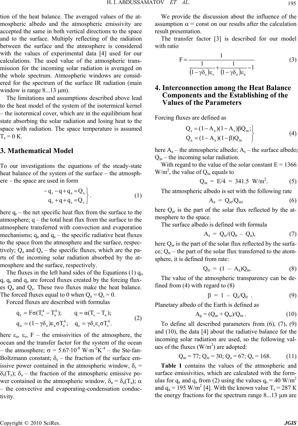

H. I. ABDUSSAMATOV ET AL.
195
tion of the heat balance. The averaged values of the at-
mospheric albedo and the atmospheric emissivity are
accepted the same in both vertical directions to the space
and to the surface. Multiply reflecting of the radiation
between the surface and the atmosphere is considered
with the values of experimental data [4] used for our
calculations. The used value of the atmospheric trans-
mission for the incoming solar radiation is averaged on
the whole spectrum. Atmospheric windows are consid-
ered for the spectrum of the surface IR radiation (main
window is range 8...13 m).
The limitations and assumptions described above lead
to the heat model of the system of the isotermical kernel
– the isotermical cover, which are in the equilibrium heat
state absorbing the solar radiation and losing heat to the
space with radiation. The space temperature is assumed
Тs = 0 К.
3. Mathematical Model
To our investigations the equations of the steady-state
heat balance of the system of the surface – the atmosph-
ere – the space are used in form





ssr
ааr
Qqqq
Qqqq . (1)
here qr – the net specific heat flux from the surface to the
atmosphere; q – the total heat flux from the surface to the
atmosphere transferred with convection and evaporation
mechanisms; qа and qs – the specific radiative heat fluxes
to the space from the atmosphere and the surface, respec-
tively; Qа and Qs – the specific fluxes, which are the pa-
rts of the incoming solar radiation absorbed by the at-
mosphere and the surface, respectively.
The fluxes in the left hand sides of the Equations (1) qr,
q, qa and qs are forced fluxes created by the forcing flux-
es Qa and Qs. These two fluxes make the heat balance.
The forced fluxes equal to 0 when Qа = Qs = 0.
Forced fluxes are described with formulas
44
rsa sa
44
aaaassss
qFσ(TT );qα(TT );
q(1γδ )εσT; qγδ ε σT.
 
 (2)
here а, s, F – the emissivities of the atmosphere, the
ocean and the transfer factor for the system of the ocean
– the atmosphere;  = 5.6710-8 Wm-2K-4 – the Ste-fan-
Boltzmann constant; s – the fraction of the surface em-
issive power contained in the atmospheric window, s =
s(Ts); а – the fraction of the atmospheric emissive po-
wer contained in the atmospheric window, a = a(Ta); 
– the convective and evaporating-condensation conduc-
tivity.
We provide the discussion about the influence of the
assumption  = const on our results after the calculation
result presentation.
The transfer factor [3] is described for our model
with ratio

1
1
1
1
1
1
F
aass




 (3)
4. Interconnection among the Heat Balance
Components and the Establishing of the
Values of the Parameters
Forcing fluxes are defined as





inaa
insas
)Q)(1A(1Q
;Q)A)(1A(1Q (4)
here Аа – the atmospheric albedo; Аs – the surface albedo;
Qin – the incoming solar radiation.
With regard to the value of the solar constant Е = 1366
W/m2, the value of Qin equals to
Qin = Е/4 = 341.5 W/m2. (5)
The atmospheric albedo is set with the following rate
Аа = Qаr/Qin, (6)
here Qаr is the part of the solar flux reflected by the at-
mosphere to the space.
The surface albedo is defined with formula
Аs = Qsr/(Qtr – Qa), (7)
here Qsr is the part of the solar flux reflected by the surfa-
ce; Qtr – the part of the solar flux transferred to the atom-
sphere, it is defined from rate:
Qtr = (1 – Аа)Qin. (8)
The value of the atmospheric transparency can be de-
fined from (4) with regard to (8)
 = 1 – Qа/Qtr . (9)
Planetary albedo of the Earth is defined as
Ap = (Qar + Qsr)/Qin . (10)
To define all described parameters from (6), (7), (9)
and (10), the data [4] about the radiative balance for the
incoming solar radiation are used, so the following val-
ues of the fluxes (W/m2) are adopted:
Qar = 77; Qsr = 30; Qa = 67; Qs = 168. (11)
Table 1 contains the values of the atmospheric and
surface emissivities, which are calculated with the form-
ulas for qa and qs from (2) using the values qs = 40 W/m2
and qa = 195 W/m2 [4]. With the known value Тs = 287 К
the energy fractions for the spectrum range 8...13 µm are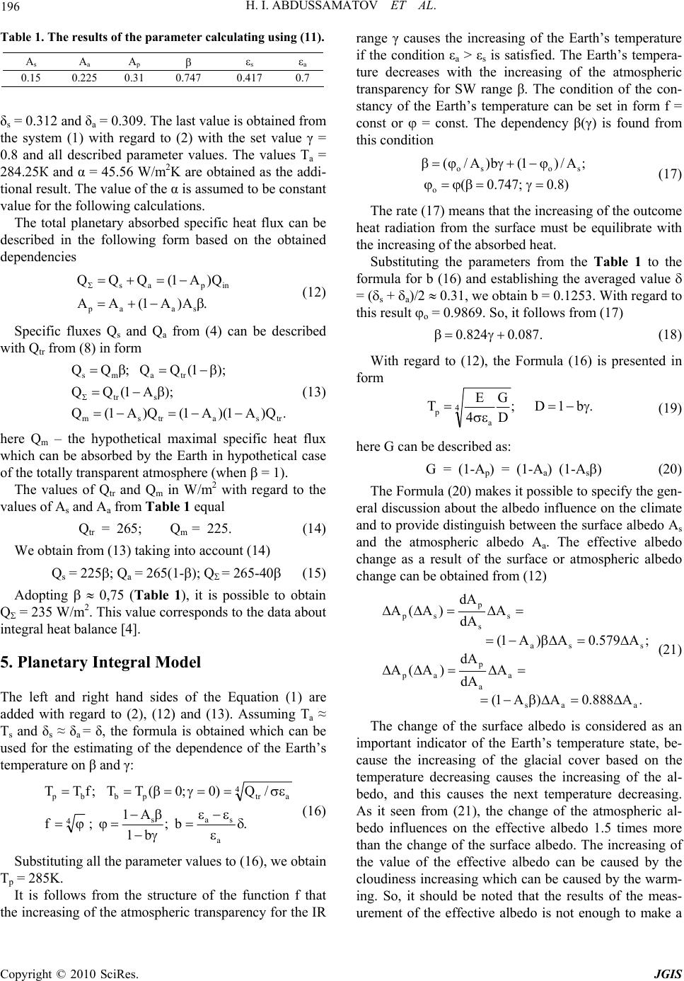

H. I. ABDUSSAMATOV ET AL.
196
Table 1. The results of the parameter calculating using (11).
Аs Аa Аp  s a
0.15 0.225 0.31 0.747 0.417 0.7
δs = 0.312 and δa = 0.309. The last value is obtained from
the system (1) with regard to (2) with the set value γ =
0.8 and all described parameter values. The values Тa =
284.25К and α = 45.56 W/m2K are obtained as the addi-
tional result. The value of the α is assumed to be constant
value for the following calculations.
The total planetary absorbed specific heat flux can be
described in the following form based on the obtained
dependencies
.A)A1(AA
Q)A1(QQQ
saap
inpas


 (12)
Specific fluxes Qs and Qa from (4) can be described
with Qtr from (8) in form
.Q)A1)(A1(Q)A1(Q
);A1(QQ
);1(QQ;QQ
trsatrsm
str
trams






 (13)
here Qm – the hypothetical maximal specific heat flux
which can be absorbed by the Earth in hypothetical case
of the totally transparent atmosphere (when  = 1).
The values of Qtr and Qm in W/m2 with regard to the
values of Аs and Аa from Table 1 equal
Qtr = 265; Qm = 225. (14)
We obtain from (13) taking into account (14)
Qs = 225; Qa = 265(1-); Q = 265-40 (15)
Adopting   0,75 (Table 1), it is possible to obtain
Q = 235 W/m2. This value corresponds to the data about
integral heat balance [4].
5. Planetary Integral Model
The left and right hand sides of the Equation (1) are
added with regard to (2), (12) and (13). Assuming Ta ≈
Ts and δs ≈ δа = δ, the formula is obtained which can be
used for the estimating of the dependence of the Earth’s
temperature on β and γ:
.b;
b1
A1
;f
/Q)0;0(TT;fTT
a
sas
4
4atrpbbp








(16)
Substituting all the parameter values to (16), we obtain
Tp = 285K.
It is follows from the structure of the function f that
the increasing of the atmospheric transparency for the IR
range γ causes the increasing of the Earth’s temperature
if the condition εa > εs is satisfied. The Earth’s tempera-
ture decreases with the increasing of the atmospheric
transparency for SW range β. The condition of the con-
stancy of the Earth’s temperature can be set in form f =
const or  = const. The dependency β(γ) is found from
this condition
)8.0;747.0(
;A/)1(b)A/(
o
soso

 (17)
The rate (17) means that the increasing of the outcome
heat radiation from the surface must be equilibrate with
the increasing of the absorbed heat.
Substituting the parameters from the Table 1 to the
formula for b (16) and establishing the averaged value 
= (s + a)/2  0.31, we obtain b = 0.1253. With regard to
this result o = 0.9869. So, it follows from (17)
.087.0824.0




(18)
With regard to (12), the Formula (16) is presented in
form
.b1D;
D
G
4
E
T4
a
p

 (19)
here G can be described as:
G = (1-Ap) = (1-Aa) (1-As) (20)
The Formula (20) makes it possible to specify the gen-
eral discussion about the albedo influence on the climate
and to provide distinguish between the surface albedo As
and the atmospheric albedo Aa. The effective albedo
change as a result of the surface or atmospheric albedo
change can be obtained from (12)
.A888.0A)A1(
A
dA
dA
)A(A
;A579.0A)A1(
A
dA
dA
)A(A
aas
a
a
p
ap
ssa
s
s
p
sp




(21)
The change of the surface albedo is considered as an
important indicator of the Earth’s temperature state, be-
cause the increasing of the glacial cover based on the
temperature decreasing causes the increasing of the al-
bedo, and this causes the next temperature decreasing.
As it seen from (21), the change of the atmospheric al-
bedo influences on the effective albedo 1.5 times more
than the change of the surface albedo. The increasing of
the value of the effective albedo can be caused by the
cloudiness increasing which can be caused by the warm-
ing. So, it should be noted that the results of the meas-
urement of the effective albedo is not enough to make a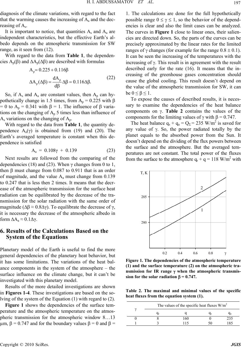

H. I. ABDUSSAMATOV ET AL.
197
diagnosis of the climate variations, with regard to the fact
that the warming causes the increasing of Aa and the dec-
reasing of As.
It is important to notice, that quantities As and Aa are
independent characteristics, but the effective Earth’s al-
bedo depends on the atmospheric transmission for SW
range, as it seen from (12).
With regard to the data from Table 1, the dependen-
cies Ap() and Аp() are described with formulas
.116.0
d
dA
)(A
116.0225.0A
p
p
p




(22)
So, if As and Aa are constant values, then Ap can hy-
pothetically change in 1.5 times, from Ap = 0.225 with 
= 0 to Аp = 0.341 with  = 1. The influence of  varia-
tions on the changing of Ap 5 times less than influence of
As variations on the changing of Ap.
With regard to the data from Table 1, the quantity de-
pendence Aa(γ) is obtained from (19) and (20). The
Earth’s averaged temperature is constant when this de-
pendence is satisfied
Aa = 0.108γ + 0.139 (23)
Next results are followed from the comparing of the
dependencies (18) and (23). When γ changes from 0 to 1,
then  must change from 0.087 to 0.911 that is an order
of magnitude, and the value Aa must change from 0.139
to 0.247 that is less then 2 times. It means that the decr-
ease of the atmospheric transmission for the surface heat
radiation can be equilibrated by the decrease of the tra-
nsmission for the solar radiation with the same order of
magnitude ( ≈ 0.8γ). To equilibrate the decrease of γ,
it is necessary the decrease of the atmospheric albedo in
form Aa ≈ 0.1Δγ.
6. Results of the Calculations Based on the
System of the Equations
Planetary model of the Earth is useful to find the more
general dependencies of the planetary heat behavior, but
it has some limitations. The variations of the heat bal-
ance components in the system of the atmosphere – the
surface influence on the climate change, but it can’t be
investigated with this planetary model.
Results of the more detailed investigations are shown
in Figures 1-4. These investigations are based on the so-
lving of the system of the Equation (1) with regard to (2).
Figure 1 shows the dependencies of the surface tem-
perature and the atmospheric temperature on the atmos-
pheric transmission for the atmospheric window 8…13
µm,  = 0.747 and for the boundary values  = 0 and  =
1. The calculations are done for the full hypothetically
possible range 0    1, so the behavior of the depend-
encies is clear and also the limit cases can be analyzed.
The curves in Figure 1 close to linear ones, their salien-
cies are directed down. So, the parts of the curves can be
precisely approximated by the linear rates for the limited
ranges of  changes (for example for the range 0.8  0.1).
It can be seen the increasing of the temperatures with the
increasing of . This result is in agreement with the result
described early for the rate (16). It means that the in-
creasing of the greenhouse gases concentration should
cause the global cooling. This result doesn’t depend on
the value of the atmospheric transmission for SW, it can
be 0 ≤  ≤ 1.
To expose the causes of described results, it is neces-
sary to examine the dependencies of the heat balance
components on . Table 2 contains the values of the
components for the limiting values of  with  = 0.747.
The heat balance qs + qa = Q = 235 W/m2 is saved for
any value of . So, the power radiated totally by the
planet equals to the absorbed power from the Sun. It
doesn’t depend on the dividing of the flux powers between
the surface and the atmosphere. But the averaged tem-
peratures are not constant. The total power of the fluxes
from the surface to the atmosphere qr + q = 118 W/m2 with
Figure 1. The dependencies of the atmospheric temperature
(1) and the surface temperature (2) on the atmospheric tra-
nsmission for IR range  when the atmospheric transmis-
sion for the solar radiation  = 0.747.
Table 2. The maximal and minimal values of the specific
heat fluxes from the equation system (1).
The values of the specific heat fluxes W/m2
 qr q qs q
a
0 8 160 0 235
1 3 115 50 185

H. I. ABDUSSAMATOV ET AL.
198
 = 1 and qr + q = 168 W/m2 with  = 0. The difference is
50 W/m2, it is the value of qs( = 1). So, the decreasing
of  causes the increasing of the power absorbed by the
atmosphere, and this power re-radiated by the atmos-
phere to the space. It causes the decreasing of the at-
mospheric temperature. As the atmosphere is the cover
for the surface, the surface is cooling too.
It is important to note that the described results are
correct when the condition а > s is performed. As cal-
culations shown, the dependencies Тs() and Та() decr-
ease in the case а < s. The condition а = s is the border
between these cases. This condition corresponds to the
value qs  60 W/m2, а = s = 0.7 and the values of all
other parameters keep constant. Actually, the decreasing
of the atmospheric transmission causes the global cool-
ing in the case of initial state  = 0.8 only when the con-
dition qs ≤ 0.25qa is satisfied.
Note, that the radiative heat transfer doesn’t take main
part in the heat transfer between the surface and the atm-
osphere. This heat transfer is mainly defined by the con-
vection and the condensation-evaporation.
Note, that the value of atmospheric transmission in
SW  influences weakly on the dependencies qs() and
qа(). Both these dependencies are quite linear, first one
is a directly proportional one qs = qm. The coefficient
equals qm = 50 W/m2 when  = 0.747. The value of qm
changes weakly – from ~49 W/m2 when  = 1 to ~56
Вт/м2 when  = 0.
The values qа for  = 0.747 and the boundary values of
 and  are shown in Table 3.
Figure 2 shows the dependencies () calculated from
the system (1) in comparison with the dependence (18).
The only one condition can be satisfied: Ts = const or Ta
= const. If any temperature is constant then another tem-
perature will change. This fact is shown in Figure 4 in
terms of quantity. It makes it impossible to keep the heat
balance for the system of the surface – the atmosphere,
so actually the compensating of the  change with the 
change isn’t possible.
Figure 3 shows the dependence of the atmospheric
albedo on  which ensure the constancy of the surface
temperature Ts (the curve 1) or the atmospheric tempe-
rature Ta (the curve 2) and also of the averaged tempera-
ture of the system of the surface – the atmosphere (dash-
Table 3. The values of the fluxes qа W/m2 radiated by the
atmosphere to the space.
The values of qа
Table
Head
 = 0  = 1  = 0.747
0 260 225 235
1 205 175 185
Figure 2. The dependence of the atmospheric transmission
for the solar radiation on the atmospheric transmission for
the surface heat radiation making the constant value Ts =
287 K (1) or Ta = 284.25 K (2). The dot line shows the de-
pendence (18).
Figure 3. The dependencies Aa() for the cases of constant
temperatures Ts (1), Ta() (2), Tp (dashed line).
ed-line curve). The mismatch of the curves 1 and 2 sh-
ows that it is impossible to compensate the  change with
the atmospheric albedo change. It causes from the data
presented in Figure 4
Results presented in Figures 2-4 have shown that pro-
jects of the scattering of the absorbing aerosol or reflect-
ing aerosol are not scientifically grounded definitely; it is
possible to provide the approach resulting to the deduc-
tion that this scattering is rather dangerous.
The assumption α = const is adopted for our calcula-
tions. It is discussed below. Generally, the convective
and evaporating coefficient α depends on the temperature

H. I. ABDUSSAMATOV ET AL.
199
Figure 4. The dependencies Ta() (1) and Ts() (2) corre-
sponding to the curve 1 and the curve 2 on Figure 2, respec-
tively.
difference ΔTsa = Ts − T
a and on the temperature level.
For the dependence α(Та) it is important that that depen-
dencies of air thermophysical properties on its tempera-
ture are weak. Calculations show the atmospheric tem-
perature change from Ta ≈ 277 K to Ta ≈ 286 K (about ~9
K) with γ change from 0 to 1. The specific air heat ca-
pacity is constant (cp = 1,005 kJ/kg K), the Prandtl num-
ber (Pr) change is less then 0,5%. Air density (ρ, kg/m3)
is decreased on ~5%, the heat conduction (λ, W/mK) is
decreased on ~5%, and the kinematic viscosity (υ, m2/s)
is increased on ~5%. Calculations based on the assump-
tion α = const show the temperature drop ΔTsa is de-
creased on ~30% (from 3,5K to 2,5K) with the increas-
ing of γ from 0 to 1.
The analysis of the equations describing the convec-
tive heat transfer with Nusselt, Grashof and Prandtl num-
bers [5] shows the decreasing of α on ~15% with the
increasing of γ from 0 to 1 with regard to mass transfer.
The behavior of the dependencies Ts(γ) and Ta(γ) with
the change of α from α = 40 W/m2K to α = 50 W/m2K
(about ~20% around the basic value 45,55 W/m2K) were
investigated. The important regularity was found. The
change of the temperatures rise isn’t more than ~0,02 K
for the range 40 ≤ α ≤ 50, so the variations of α causes
the calculating error about 0,2%. It can be concluded that
the heat transfer between the surface and the atmosphere
influences on the dependencies Ts(γ) and Ta(γ) weakly.
These dependencies are mostly determinated by the ra-
diative balance and by the change of the radiative heat
fluxes from the surface and the atmosphere to the space.
The value of α establishes the basic value of the tem-
perature Ta with the set value of Ts. It indicates on the
possibility to use the assumption α = const for the inves-
tigations of the surface and atmospheric temperature de-
pendencies on the atmospheric transmission.
7. Conclusions
● The decreasing of the atmospheric transmission for the
surface radiation should cause the global cooling with the
set of the parameters of the system of the surface – the
atmosphere. So, the conception of the increasing of the
greenhouse gases concentration and, as a result, the
warming is required to be revisited. Small variations of
the heat balance [6] for the system of the surface – the
atmosphere don’t influence on the described results. Ob-
tained results are in good agreement with the results from
the work [7];
● the Earth’s effective albedo are defined by the val-
ues of the atmospheric and surface albedo and by the
atmospheric transmission for the solar radiation as well;
the effective albedo seems as a mixed criteria of the cli-
mate state;
● the indemnity of the change of the atmospheric tra-
nsmission for the surface radiation with the change of the
transmission for the incoming solar radiation or the at-
mospheric albedo doesn’t look as a possible action. The
attempts to use the reflecting aerosols or absorbing aero-
sols are the dangerous operations.
Some additional remarks:
● The behavior of the temperature dependencies on 
is independent from taking into account all atmospheric
windows or ignoring some of them. And more, assuming
δ = 1, we didn’t find the quality changes of the depend-
encies Ts() and Tа(). Calculations have shown the in-
creasing of the temperatures with the increasing of γ for
the spectrum range 13…17.5 m, where the surface ra-
diation is almost totally absorbed by carbon dioxide and
water vapor.
● Calculations for the hypothetically possible range 0
   1 make it possible to find the behavior of the de-
pendencies Ts() and Ta(). These dependencies are mo-
notony. Note that the limitation of the range of the possi-
ble transmission variations can reach to the incorrect
results. In particular, the assumption q = const can be
accepted to solve the system (1), but it can be seen for
the full range of  change that the dependencies Ts() and
Ta() intersect each other, i.e., the convective-evaporative
flux q is changed and it’s sigh is changed. Last result
contradicts to the assumption q = const. But for the case
q = const the calculations shows the increasing of the
surface temperature caused by the decreasing of the
transmission for the surface IR radiation.

H. I. ABDUSSAMATOV ET AL.
200
8. References
[1] S. Manabe and R. F. Strickler, “Thermal Equilibrium of
the Atmosphere with a Convective Adjustment,” Journal
of Atmospheric Science, Vol. 21, Vol. 6, 1964, pp. 361-
385.
[2] V. Ramanathan, “The Role of Ocean-Atmosphere Inter-
actions in the CO2 Climate Problem,” Journal of Atmos-
pheric Science, Vol. 38, Vol. 5, 1981, pp. 918-930.
[3] H. John, I. V. Lienhard and V. Lienhard, “A Heat Trans-
fer Textbook,” 3rd Edition, Phlogiston Press, Cambridge,
2008.
[4] J. T. Keihl and K. E. Trenberth, “Earth’s Annual
Global Mean Energy Budget,” Bulletin of the American
Meteorological Society, Vol. 78, No. 2, 1997, pp. 97-208.
[5] E. R. G. Ekkert and R. M. Drake, Jr., “Analysis of Heat
and Mass Transfer,” Hemisphere Publishing Corp.,
Washington, D.C., 1987.
[6] K. E. Trenberth, J. T. Fasullo and J. T. Keihl, “Earth’s
Global Energy Budget,” Bulletin of the American Mete-
orological Society, Vol. 90, No. 3, 2009, pp. 311-323.
[7] G. V. Chilingar, L. F. Khilyuk and O. G. Sorokhtin, “Co-
oling of Atmosphere Due to CO2 Emission,” Energy So-
urces, Part A: Recovery, Utilization, and Environmental
Effects, Vol. 30, No. 1, 2008, pp. 1-9.