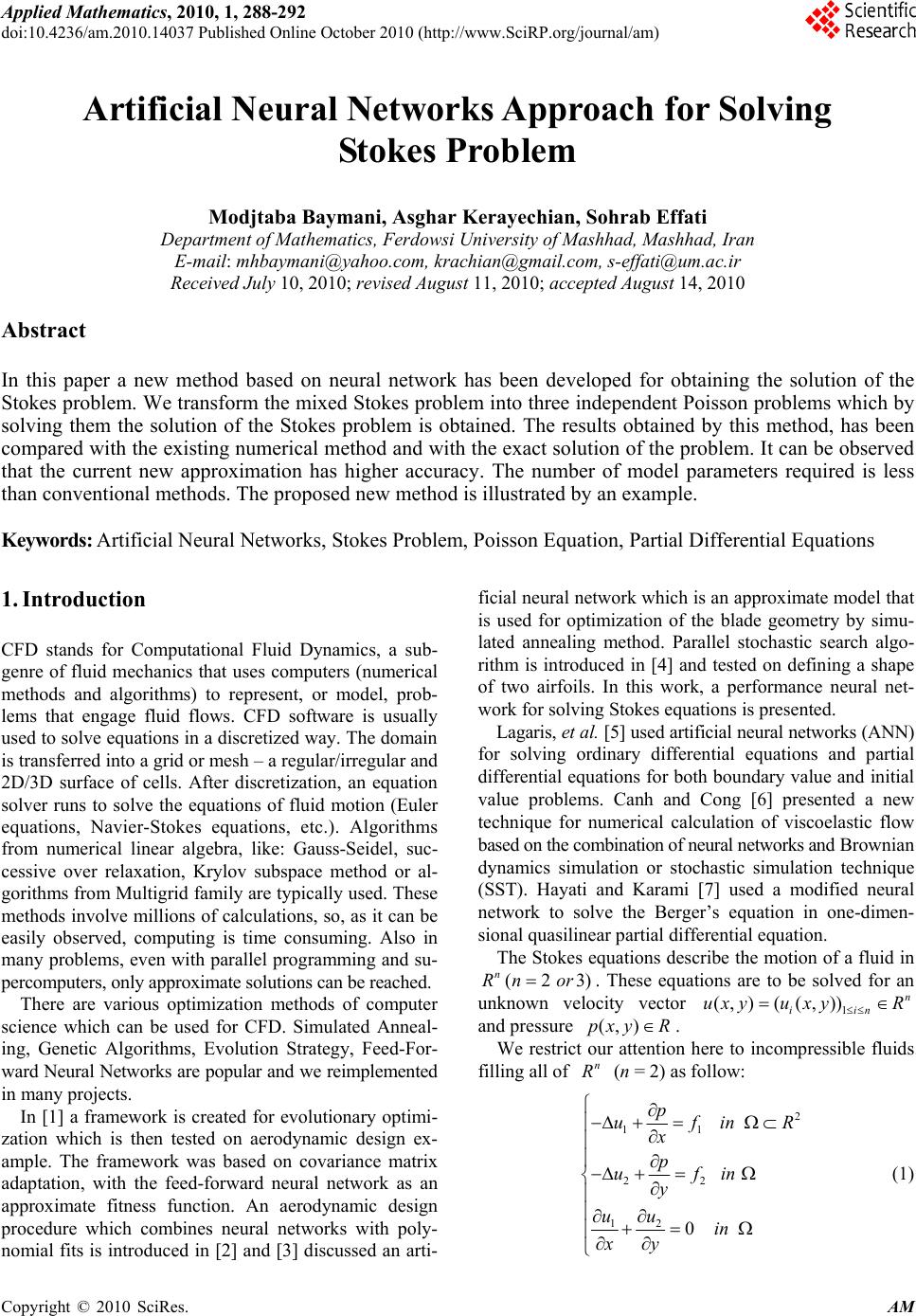Applied Mathematics, 2010, 1, 288-292
doi:10.4236/am.2010.14037 Published Online October 2010 (http://www.SciRP.org/journal/am)
Artificial Neural Networks Approach for Solving
Stokes Problem
Modjtaba Baymani, Asghar Kerayechian, Sohrab Effati
Department of Mathematics, Ferdowsi University of Mashhad, Mashhad, Iran
Received July 10, 2010; revised August 11, 2010; accepted August 14, 2010
Abstract
In this paper a new method based on neural network has been developed for obtaining the solution of the
Stokes problem. We transform the mixed Stokes problem into three independent Poisson problems which by
solving them the solution of the Stokes problem is obtained. The results obtained by this method, has been
compared with the existing numerical method and with the exact solution of the problem. It can be observed
that the current new approximation has higher accuracy. The number of model parameters required is less
than conventional methods. The proposed new method is illustrated by an example.
Keywords: Artificial Neural Networks, Stokes Problem, Poisson Equation, Partial Differential Equations
1. Introduction
CFD stands for Computational Fluid Dynamics, a sub-
genre of fluid mechanics that uses computers (numerical
methods and algorithms) to represent, or model, prob-
lems that engage fluid flows. CFD software is usually
used to solve equations in a discretized way. The domain
is transferred into a grid or mesh – a regular/irregular and
2D/3D surface of cells. After discretization, an equation
solver runs to solve the equations of fluid motion (Euler
equations, Navier-Stokes equations, etc.). Algorithms
from numerical linear algebra, like: Gauss-Seidel, suc-
cessive over relaxation, Krylov subspace method or al-
gorithms from Multigrid family are typically used. These
methods involve millions of calculations, so, as it can be
easily observed, computing is time consuming. Also in
many problems, even with parallel programming and su-
percomputers, only approximate solutions can be reached.
There are various optimization methods of computer
science which can be used for CFD. Simulated Anneal-
ing, Genetic Algorithms, Evolution Strategy, Feed-For-
ward Neural Networks are popular and we reimplemented
in many projects.
In [1] a framework is created for evolutionary optimi-
zation which is then tested on aerodynamic design ex-
ample. The framework was based on covariance matrix
adaptation, with the feed-forward neural network as an
approximate fitness function. An aerodynamic design
procedure which combines neural networks with poly-
nomial fits is introduced in [2] and [3] discussed an arti-
ficial neural network which is an approximate model that
is used for optimization of the blade geometry by simu-
lated annealing method. Parallel stochastic search algo-
rithm is introduced in [4] and tested on defining a shape
of two airfoils. In this work, a performance neural net-
work for solving Stokes equations is presented.
Lagaris, et al. [5] used artificial neural networks (ANN)
for solving ordinary differential equations and partial
differential equations for both boundary value and initial
value problems. Canh and Cong [6] presented a new
technique for numerical calculation of viscoelastic flow
based on the combination of neural networks and Brownian
dynamics simulation or stochastic simulation technique
(SST). Hayati and Karami [7] used a modified neural
network to solve the Berger’s equation in one-dimen-
sional quasilinear partial differential equation.
The Stokes equations describe the motion of a fluid in
(23)
n
Rn or. These equations are to be solved for an
unknown velocity vector 1 (, )((, ))n
iin
uxyu xyR


and pressure (, )pxy R

.
We restrict our attention here to incompressible fluids
filling all of n R (n = 2) as follow:
2
11
22
12
0
p
ufinR
x
p
ufin
y
uu in
xy

 



 



 


(1)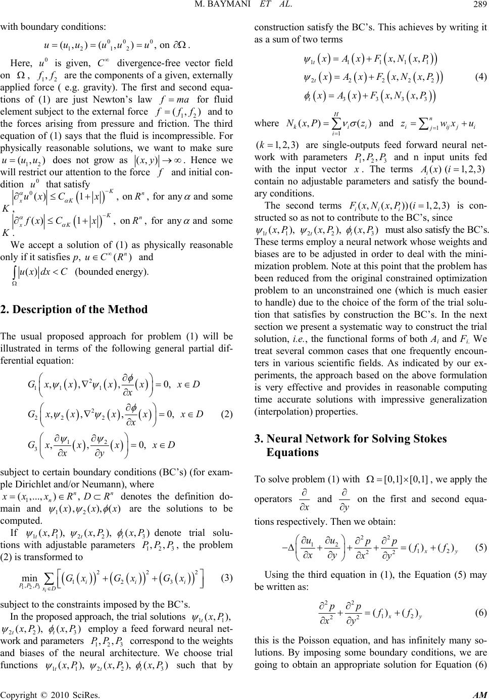

M. BAYMANI ET AL. 289
with boundary conditions:
00 0
121 2
(, ) (,),onuuu uuu .
Here, 0
u is given, C divergence-free vector field
on , 12 ,
f
f are the components of a given, externally
applied force ( e.g. gravity). The first and second equa-
tions of (1) are just Newton’s law
f
ma for fluid
element subject to the external force 12 (, )
f
ff and to
the forces arising from pressure and friction. The third
equation of (1) says that the fluid is incompressible. For
physically reasonable solutions, we want to make sure
12
(, )uuu does not grow as (,)xy . Hence we
will restrict our attention to the force
f
and initial con-
dition 0 u that satisfy

0() 1
K
xK
ux Cx



, onn
R, for any

and some
K,

() 1
K
xK
fx Cx



, onn
R, for any

and some
K.
We accept a solution of (1) as physically reasonable
only if it satisfies,()
n
pu CR

 and
()ux dxC


 (bounded energy).
2. Description of the Method
The usual proposed approach for problem (1) will be
illustrated in terms of the following general partial dif-
ferential equation:

 
 
2
11 1
2
22 2
12
3
,,,0,
,,,0,
,,0,
Gx xxxxD
x
Gx xxxxD
x
GxxxxD
xy


















 



(2)
subject to certain boundary conditions (BC’s) (for exam-
ple Dirichlet and/or Neumann), where
1
( ,...,),
nn
n
x
xxRDR denotes the definition do-
main and 12 (), (),()
x
xx

 are the solutions to be
computed.
If 112 23 (,), (,), (,)
ttt
x
PxPxP

 denote trial solu-
tions with adjustable parameters 123 ,,PPP, the problem
(2) is transformed to
     
123
222
123
,,
min
i
iii
PPPxD
Gx Gx Gx





 (3)
subject to the constraints imposed by the BC’s.
In the proposed approach, the trial solutions 11 (, ),
t
x
P

22 3
(,), (,)
tt
x
PxP

 employ a feed forward neural net-
work and parameters 123
,,PPP correspond to the weights
and biases of the neural architecture. We choose trial
functions 11223
(,), (,), (,)
ttt
x
PxPxP

 such that by
construction satisfy the BC’s. This achieves by writing it
as a sum of two terms



 
 

   
11111
22222
3333
,,
,,
,,
t
t
t
xAxFxNxP
x
Ax FxNxP
xAxFxNxP






(4)
where
1
(, )( )
H
kii
i
NxPz 

 and 1
n
iijji
j
zwxu



(1,2,3)k

are single-outputs feed forward neural net-
work with parameters 123
,,PPP and n input units fed
with the input vector
x
. The terms ()(1,2,3)
i
Ax i

contain no adjustable parameters and satisfy the bound-
ary conditions.
The second terms (,(,))(1,2,3)
iii
FxNxP i is con-
structed so as not to contribute to the BC’s, since
112 23
(,), (,), (,)
ttt
x
PxPxP

 must also satisfy the BC’s.
These terms employ a neural network whose weights and
biases are to be adjusted in order to deal with the mini-
mization problem. Note at this point that the problem has
been reduced from the original constrained optimization
problem to an unconstrained one (which is much easier
to handle) due to the choice of the form of the trial solu-
tion that satisfies by construction the BC’s. In the next
section we present a systematic way to construct the trial
solution, i.e., the functional forms of both Ai and Fi. We
treat several common cases that one frequently encoun-
ters in various scientific fields. As indicated by our ex-
periments, the approach based on the above formulation
is very effective and provides in reasonable computing
time accurate solutions with impressive generalization
(interpolation) properties.
3. Neural Network for Solvi n g S t o k e s
Equations
To solve problem (1) with [0,1] [0,1]

, we apply the
operators
x


and y


on the first and second equa-
tions respectively. Then we obtain:
22
12
12
22
() ()
x
y
uu pp
f
f
xy xy
 
 

 
 (5)
Using the third equation in (1), the Equation (5) may
be written as:
22
12
22
() ()
x
y
pp
f
f
xy

 
 (6)
this is the Poisson equation, and has infinitely many so-
lutions. By imposing some boundary conditions, we are
going to obtain an appropriate solution for Equation (6)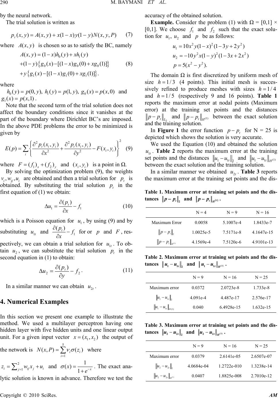

M. BAYMANI ET AL. 290
by the neural network.
The trial solution is written as
),,()1()1(),(),( PyxNyyxxyxAyxpt (7)
where (, )
A
xy is chosen so as to satisfy the BC, namely


01
000
111
(, )(1)()()
(1)()[(1)(0)(1)]
() [(1)(0)(1)].
Axyxhyxh y
ygxxg xg
ygxxg xg
 
 

(8)
where
010
()(0,), ()(1,), ()(,0)hypy hypygxpx and
1() (,1)
g
xpx.
Note that the second term of the trial solution does not
affect the boundary conditions since it vanishes at the
part of the boundary where Dirichlet BC’s are imposed.
In the above PDE problems the error to be minimized is
given by
2
22
22
(, )(, )
()( ,)
tiitii ii
i
pxy pxy
EpFx y
xy








 (9)
where 12
()( )
x
y
F
ff and (, )
ii
x
y is a point in Ω.
By solving the optimization problem (9), the weights
,,
iiji
vwu are obtained and then a trial solution for t p is
obtained. By substituting the trial solution t p in the
first equation of (1) we obtain:
11
()
t
p
uf
x

 
 (10)
which is a Poisson equation for 1 u, by using (9) and by
substituting 1t u and 1
()
t
p
f
x

 for or p and
F
, res-
pectively, we can obtain a trial solution for 1t u. To ob-
tain 2 u, we can substitute the trial solution t p in the
second equation in (1) to obtain:
22
)( f
y
p
ut


 . (11)
In a similar manner we can obtain 2t
u.
4. Numerical Examples
In this section we present one example to illustrate the
method. We used a multilayer perceptron having one
hidden layer with five hidden units and one linear output
unit. For a given input vector 12 (,)
x
xx the output of
the network is
5
1
(, )( )
ii
i
NxP z 

 where
2
1
iijji
j
zwxu


 and 1
() 1
x
xe 

. The exact ana-
lytic solution is known in advance. Therefore we test the
accuracy of the obtained solution.
Example. Consider the problem (1) with Ω = [0,1] ×
[0,1]. We choose 1 f and 2 f such that the exact solu-
tion for 12 ,uu and p be as follows:
22 2
1
222
2
22
10(1) (132)
10(1) (132)
5( ).
uxyx yy
uyxyxx
pxy

 

The domain Ω is first discretized by uniform mesh of
size 1/3h

(4 points). This initial mesh is succes-
sively refined to produce meshes with sizes 1/4h

and 1/5h

(respectively 9 and 16 points). Table 1
reports the maximum error at nodal points (Maximum
error) at the training set points and the distances
2
t
L
pp and (1)
tH
pp between the exact solution
and the training solution.
In Figure 1 the error function t pp for N = 25 is
depicted which shows the solution is very accurate.
We used the Equation (10) and obtained the solution
1t
u. Table 2 reports the maximum error at the training
set points and the distances 11
2
t
uu and (1)
11tH
uu
between the exact solution and the training solution.
In a similar manner we obtained 2t u. Table 3 reports
the maximum error at the training set points and the dis-
Table 1. Maximum error at training set points and the dis-
tances 2
t
pp and 1
tH
pp() .
N = 16 N = 9 N = 4
1.8433e-75.1007e-4 0.0058 Maximum Error
4.1647e-157.5171e-8 1.0025e-5
2
t
p
p
4.9101e-137.5120e-6 4.1569e-4
(1)
tH
pp
Table 2. Maximum error at training set points and the dis-
tances 
11
2
t
uu and () 1
11tH
uu .
N = 25 N = 16 N = 9
1.733e-8 2.0723e-8 0.0372 Maximum error
2.576e-17 4.487e-17 4.091e-4
11
2
t
uu
1.632e-15 6.4928e-15 0.040
11
(1)
tH
uu
Table 3. Maximum error at training set points and the dis-
tances 
22
2
t
uu and () 1
22tH
uu .
N = 25 N = 16 N = 9
2.6507e-072.6141e-05 0.0379 Maximum error
1.3238e-141.2722e-010 4.0684e-04
22
2
t
uu
2.7010e-121.8825e-008 0.0407 (1)
22tH
uu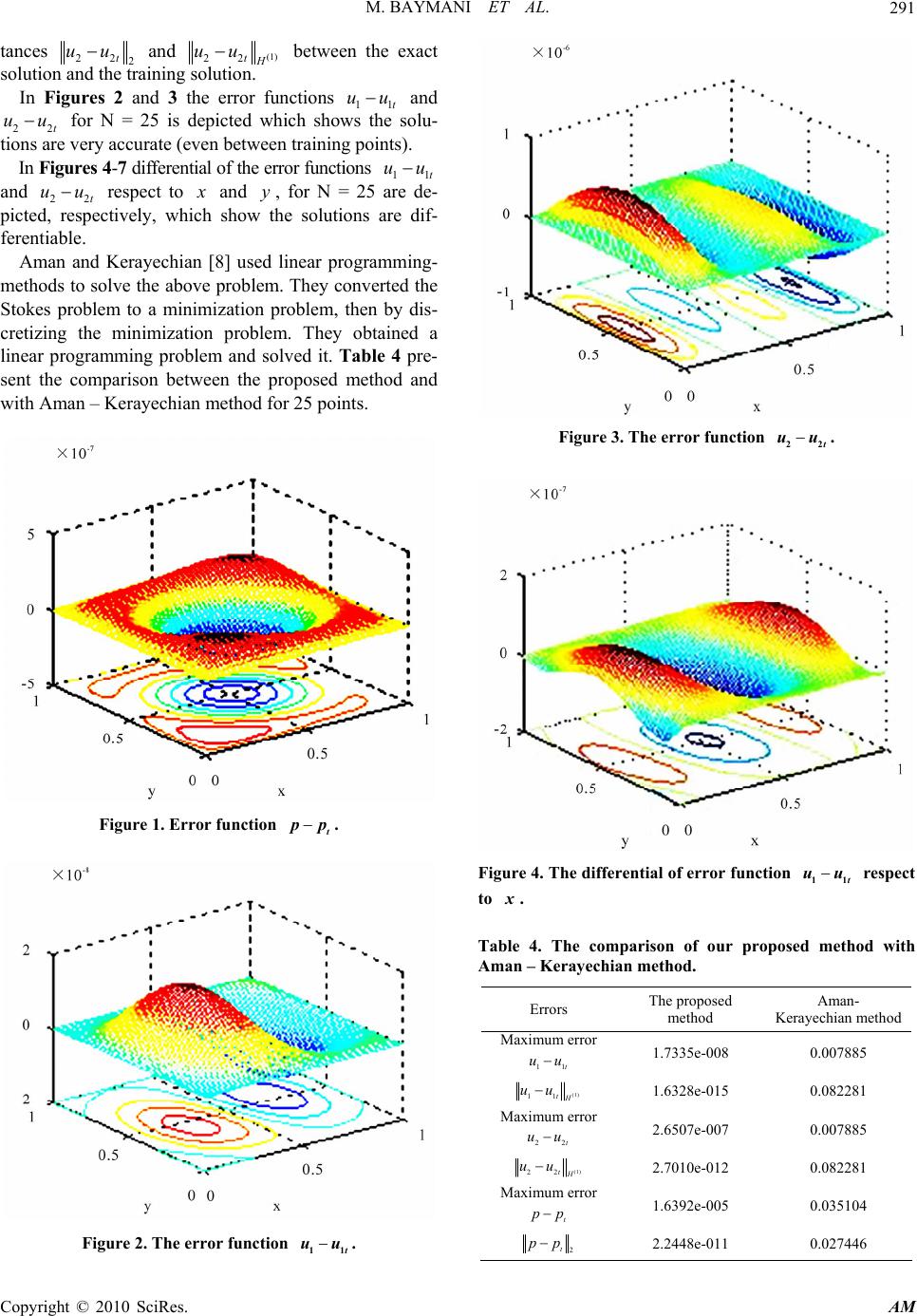

M. BAYMANI ET AL. 291
tances 22
2
t
uu and (1)
22tH
uu between the exact
solution and the training solution.
In Figures 2 and 3 the error functions 11t uu

and
22t
uu for N = 25 is depicted which shows the solu-
tions are very accurate (even between training points).
In Figures 4-7 differential of the error functions 11t uu

and 22t uu respect to
x
and y, for N = 25 are de-
picted, respectively, which show the solutions are dif-
ferentiable.
Aman and Kerayechian [8] used linear programming-
methods to solve the above problem. They converted the
Stokes problem to a minimization problem, then by dis-
cretizing the minimization problem. They obtained a
linear programming problem and solved it. Table 4 pre-
sent the comparison between the proposed method and
with Aman – Kerayechian method for 25 points.
Figure 1. Error function t pp.
Figure 2. The error function 
11t
uu.
Figure 3. The error function 
22t
uu.
Figure 4. The differential of error function 
11t
uu respect
to x.
Table 4. The comparison of our proposed method with
Aman – Kerayechian method.
Errors The proposed
method
Aman-
Kerayechian method
Maximum error
11t
uu

1.7335e-008 0.007885
(1)
11tH
uu 1.6328e-015 0.082281
Maximum error
22t
uu

2.6507e-007 0.007885
(1)
22tH
uu 2.7010e-012 0.082281
Maximum error
t
p
p

1.6392e-005 0.035104
2
t
p
p 2.2448e-011 0.027446

M. BAYMANI ET AL. 292
Figure 5. The differential of error function 
11t
uu respect
to y.
Figure 6. The differential of error function 
22t
uu respect
to x.
5. Conclusions
In this paper a new method based on ANN has been ap-
plied to find solution for Stokes equation. The solution
via ANN method is a differentiable, closed analytic form
easily used in any subsequent calculation. The neural
network here allows us to obtain fast solution of Stokes
equation starting from randomly sampled data sets and
refined it without wasting memory space and therefore
reducing the complexity of the problem.
If we compare the results of the numerical methods
(see [8]) with our method, we see that our method has
some small error. Other advantage of this method, the
solution of the Stokes problem is available for each arbi-
trary point in training interval (even between training
points). Indeed, after solving the Stokes problem, we
Figure 7. The differential of error function 
22t
uu respect
to y.
obtain an approximated function for the solution and so
we can calculate the answer at every point immediately.
6. References
[1] Y. C. Jin, M. Olhofer and B. Sendhoff, “A Framework
for Evolutionary Optimization with Approximate Fitness
Functions, Evolutionary Computation,” IEEE Transac-
tions, Vol. 6, No. 5, 2002, pp. 481-494.
[2] M. H. Man, R. Nateri and K. Madavan, “Aerodynamic
Design Using Neural Networks,” American Institute of
Aeronautics and Astronautics Journal, Vol. 38, No. 1,
2000, pp. 173-182.
[3] S. Pierret, “Turbo Machinery Blade Design Using a Na-
vier-Stokes Solver and Artificial Neural Network,” ASME
Journal of Turbomach, Vol. 121, No. 3, 1999, pp. 326-
332.
[4] T. Ray, H. Tsai and C. Tan, “Effects of Solver Fidelity on
a Parallel Search Algorithm’s Performance for Airfoil
Shape Optimization Problems,” 9th AIAA/ISSMO Sympo-
sium on Multidisciplinary Analysis and Optimization,
Atlanta, Georgia, 2002, pp. 1816-1826.
[5] I. E. Largris and A. Likas, “Artificial Neural Networks
for Solving Ordinary and Partial Differential Equations,”
IEEE transaction on neural networks, Vol. 9, No. 5, 1998,
pp. 987-1000.
[6] D. Tran-Canh and T. Tran-Cong, “Computation of Vis-
coelastic Flow Using Neural Networks and Stochastic
Simulation,” Korea-Australia Rheology Journal, Vol. 14,
No. 4, 2002, pp. 161-174.
[7] M. Hayati and B. Karami, “Feedforward Neural Network
for Solving Partial Differential Equations,” Journal of
Applied Sciences, Vol. 7, No. 19, 2007, pp 2812-2817.
[8] M. Aman and A. Kerayechian, “Solving the Stokes Prob-
lem by Linear Programming Methods,” International
Mathematical Journal , Vol. 5, No. 1, 2004, pp. 9-22.