Applied Mathematics, 2010, 1, 251-259
doi:10.4236/am.2010.14031 Published Online October 2010 (http://www.SciRP.org/journal/am)
Some Models of Reproducing Graphs:
II Age Capped Vertices
Richard Southwell, Chris Cannings
School of Mathematics and Statistics, University of Sheffield, Sheffield, United Kingdom
Received June 26 , 20 10; revised August 10, 2010; accepted August 12, 2010
Abstract
In the prequel to this paper we introduced eight reproducing graph models. The simple idea behind these
models is that graphs grow because the vertices within reproduce. In this paper we make our models more
realistic by adding the idea that vertices have a finite life span. The resulting models capture aspects of sys-
tems like social networks and biological networks where reproducing entities die after some amount of time.
In the 1940’s Leslie introduced a population model where the reproduction and survival rates of individuals
depends upon their ages. Our models may be viewed as extensions of Leslie’s model-adding the idea of net-
work joining the reproducing individuals. By exploiting connections with Leslie’s model we are to describe
how many aspects of graphs evolve under our systems. Many features such as degree distributions, number
of edges and distance structure are described by the golden ratio or its higher order generalisations.
Keywords: Reproduction, Graph, Population, Leslie, Golden Ratio
1. Introduction
Networks are everywhere, wherever a system can be t h o u g h t
of as a collection of discrete elements, link ed up in some
way, networks occur. With the acceleration of infor-
mation technology more and more attention is being paid
to the structure of these netwo rks, and this has led to the
proposal of many models [1-3].
In many situations networks grow-expanding in size as
material is produced from the inside, not added from
outside. To study network growth we introduced a class
of pure r eproduction models [4,5 ], where networks grow
because the vertices within reproduce. These models can
be applied to many situations where entities are intro-
duced which derive their connections from pre existing
elements. Most obviously they could be used to model
social networks, collaboration networks, networks within
growing organisms, the internet and protein-protein int erac tion
networks. One of our systems (model 3) has also been
introduced independently [6], proposed as a model for
the growth of online social networks.
In our pure reproduction models networks grow
endlessly in a deterministic fashion. This allows a rigo-
rous analysis, but costs a degree of realism. Nature in-
cludes birth and death and entities may be destroyed for
reasons of conflict, crowding or old age. In this paper we
consider age; and extend our models by including vertex
mortality.
2. The Models
In [5] we defined a set {: {0,1,,7}}
m
Fm of eight
different functions m
F
which map graphs to graphs.
()
m
F
G is the graph obtained by simultaneously giving
each of G’s vertices an offspring vertex and then
adding edges according to some rule. The connections
given to offspring depend upon the binary representation



of m (i.e. =4 2m



) as follows:
=1


offspring are connected to their parent’s
neighbours,
=1


offspring are connected to their parents,
=1


offspring are connected to their parent’s
neighbour’s of fsp ri n g.
In our age capped reproduction models we think of the
vertices as having ages. Graphs grow under these models
exactly as before, except that vertices grow and then die
when their age exceeds some pre-specified integer Q.
Our new update operator ,mQ
T is defined so that ,()
mQ
TG
is the graph obtained by taking the graph G and perfor-
ming the following process;

R. SOUTHWELL ET AL. 252
1) Increase the age of each vertex by one.
2) Give every vertex an age zero offspring, born with
connectivity dependant upon m, as above (i.e. the new
graph is ()
m
F
G).
3) Remove every vertex with age greater than the age
cap Q.
We are interested in the sequence }{ t G of graphs
which evolve from an initial structure 000 =( ,)GVE in
such a way that 1, =()
tmQt
GTG
,0t . We always
suppose that initial vertices have age Q.
3. The Number of Vertices
The number of vertices ||
t
G in t G is deeply connected
with the golden ratio and its generalisations. The number
t
i
n of age i vertices in t G can be conveniently descri-
bed in terms of Leslie matrices.
In Leslie’s population model [7,8] individuals of age
i have a survival rate i s and fertility rate i f. The
expected number of individuals of a given age, at a given
time, is kept track of via repeated multiplication of the
state vector with the ‘Leslie matrix’
012
0
1
00 0
00 0
.
00 0
Q
Q
f
ff f
s
s
s













In our case 1=.
tt
nLn
 where

01
=,,,T
ttt t
Q
nnn n
and L is the Leslie matrix with ==1
ii
sf , i

.
L is a primitive matrix with characteristic polyno-
mial
1
=0
=
QiQ
i
x
x

and principle eigenvalue Q

(also known as the 1Q

step
Fibbonacci constant). The golden ratio is 1/2
115
=2

,
2=1.8393

,3=1.9276

,4=1.9655 9

and2
Q

 as
Q. When t is large 1=
tt
Q
nn

 where
 

12
=1, ,,,T
Q
tQQ Q
nc  
 
 is the stable age
distribution and c is a constant which depends upon the
initial state of the system.
Let ,0 ,1,
= (,,...,)T
iii iQ
d   where ji,

is the Krone-
cker delta. The n step Fibonacci numbers []n
i
f
are
natural generalisations of the famous Fibonacci numbers
[9] which can be generated by repeatedly multiplying
0
d by L. When 0 G is age zero (i.e. all its vertices have
zero age)

00
=| |.
tt
ii
nGLd, where

[1]
01
.=
tQ
ti
i
Ld f


. In
such a case t G will have [1]
02
||.
Q
t
Gf

 vertices.
4. Binary Strings
As we update our graphs, their vertex sets will grow, and
a good way to keep track of these vertex sets is to use
binary strings. Suppose v is a vertex of 0
G. When we
update G we write (,0)v and (,1)v to denote v‘s
offspring, and v itself (respectively), in the graph 1
G.
This means, for example, that (( ,0),0)v is the grand
child of ((,1),1)v in 2
G. We use short hand by omit-
ting the parenthesis, so for example we write ,0),0)((v
as 00v. An example of the evolution of model 2 is
shown in Figure 1.
When our age cap =Q

an initial graph 000 =( ,)GVE
will evolve in exactly the same way as in pure repro-
duction i.e. 0
=()
t
tm
GFG ; this will have vertex set
0{0,1}t
V and edge set as specified in [5]. When Q is
finite the situation is more complex, but our binary string
notation allows us to keep track of the ages of vertices in
a convenient way.
Let ab denote the concatenation of binary strings a
and b and let t
a denote th e string obtained by conca-
tenating a with itself t times. Suppose (01)
n
va is a
vertex of t
G for some 1
{0,1}tn a . Now (0)va is a
new born offspring in tn G

and every subsequent 1 in
(01)
n
va ’s name corresponds to an update within which
Figure 1. A depiction of the evolution of model 2 when
=2Q, starting with an isolated vertex named
p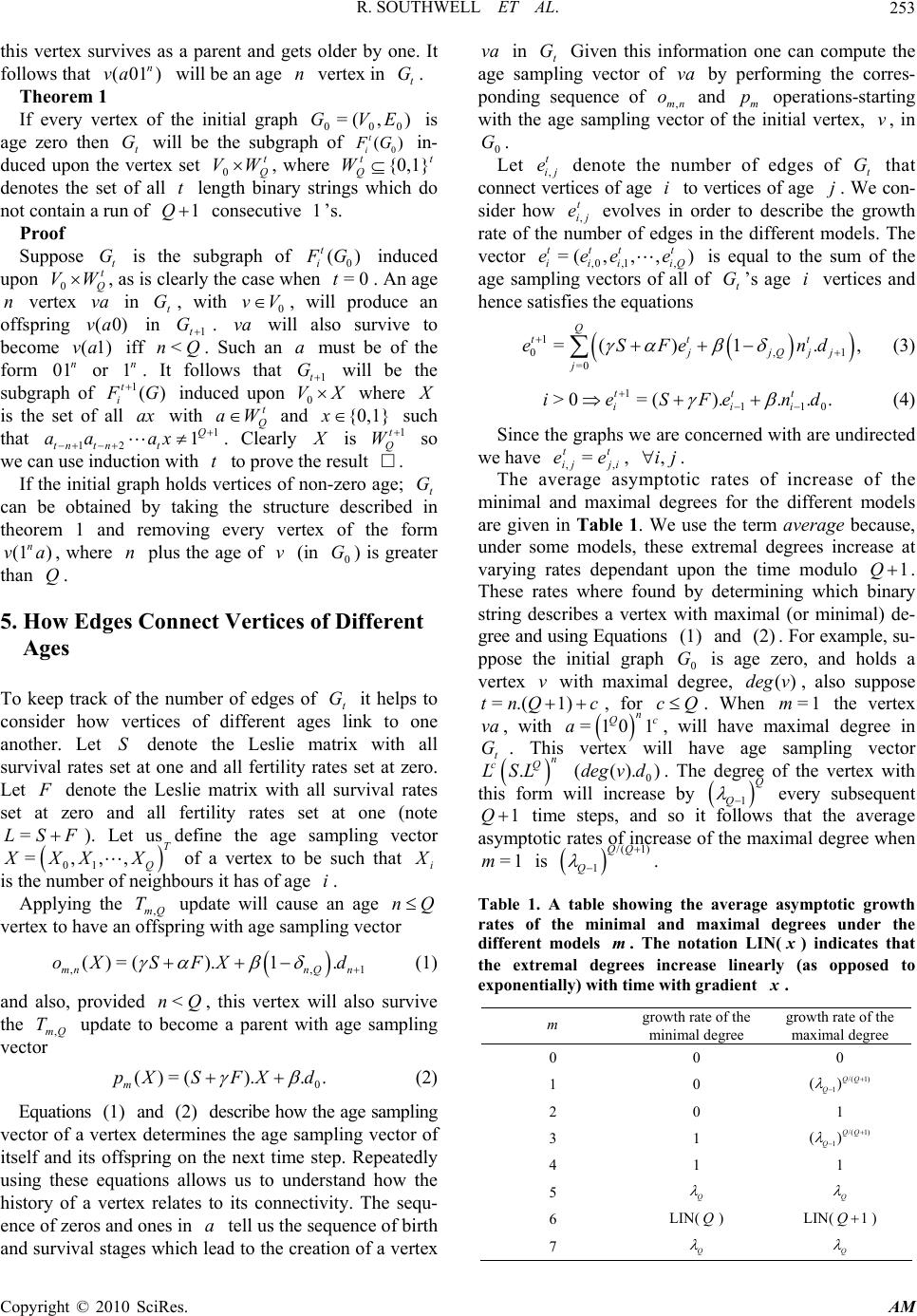
.

R. SOUTHWELL ET AL. 253
this vertex survives as a parent and gets older by one. It
follows that (01)
n
va will be an age n vertex in t G.
Theorem 1
If every vertex of the initial graph ),(= 000 EVG is
age zero then t
G will be the subgraph of 0 ()
t
i
FG in-
duced upon the vertex set t
Q
WV 
0, where tt Q
W{0,1}
denotes the set of all t length binary strings which do
not contain a run of 1Q consecutive 1’s.
Proof
Suppose t
G is the subgraph of 0
()
t
i
F
G induced
upon 0t
Q
VW, as is clearly the case when =0t. An age
n vertex va in t G, with 0 vV, will produce an
offspring (0)va in 1t
G. va will also survive to
become (1)va iff <nQ
. Such an a must be of the
form 01n or 1n. It follows that 1t
G will be the
subgraph of 1()
t
i
F
G
 induced upon 0
VX where
X
is the set of all ax with t
Q
Wa and {0,1}x such
that 1
12 1Q tn tnt
aaax
 . Clearly
X
is 1t
Q
W

so
we can use induction with
t
to prove the result .
If the initial graph holds vertices of non-zero age; t
G
can be obtained by taking the structure described in
theorem 1 and removing every vertex of the form
(1 )
n
va , where n plus the age of v (in 0 G) is greater
than Q.
5. How Edges Connect Vertices of Different
Ages
To keep track of the number of edges of t G it helps to
consider how vertices of different ages link to one
another. Let S denote the Leslie matrix with all
survival rates set at one and all fertility rates set at zero.
Let
F
denote the Leslie matrix with all survival rates
set at zero and all fertility rates set at one (note
FSL =). Let us define the age sampling vector

01
=,,,T
Q
XXXX of a vertex to be such that i X
is the number of neighbours it has of age i.
Applying the Qm
T, update will cause an age Qn

vertex to have an offspring with age sampling vector

,,1
()=(). 1 .
mnnQn
oXS FXd  

 (1)
and also, provided Qn <, this vertex will also survive
the Qm
T, update to become a parent with age sampling
vector
0
()=()...
m
pXSFXd

 (2)
Equations (1) and (2) describe how the age sampling
vector of a vertex determines the age sampling vector of
itself and its offspring on the next time step. Repeatedly
using these equations allows us to understand how the
history of a vertex relates to its connectivity. The sequ-
ence of zeros and ones in a tell us the sequence of birth
and survival stages which lead to the creation of a vertex
va in t G Given this information one can compute the
age sampling vector of va by performing the corres-
ponding sequence of ,mn o and m p operations-starting
with the age sampling vector of the initial vertex, v, in
0
G.
Let ,
t
ij
e denote the number of edges of t G that
connect vertices of age i to vertices of age j. We con-
sider how tji
e, evolves in order to describe the growth
rate of the number of edges in the different models. The
vector ,0 ,1,
=(,, ,)
ttt t
iii iQ
eee e is equal to the sum of the
age sampling vectors of all of t G’s age i vertices and
hence satisfies the equations


1
0,1
=0
=()1. ,
Q
ttt
jjQjj
j
eSFe nd 



 (3)
1110
>0=()... .
ttt
iii
ieSFend 


 (4)
Since the graphs we are concerned with are undirected
we have tij
tji ee ,,=, ji,

.
The average asymptotic rates of increase of the
minimal and maximal degrees for the different models
are given in Table 1. We use the term average because,
under some models, these extremal degrees increase at
varying rates dependant upon the time modulo 1

Q.
These rates where found by determining which binary
string describes a vertex with maximal (or minimal) de-
gree and using Equations (1) and (2). For example, su-
ppose the initial graph 0 G is age zero, and holds a
vertex v with maximal degree, ()deg v, also suppose
=.(1)tnQ c

, for Qc

. When =1m the vertex
va , with

=101
n
Qc
a, will have maximal degree in
t
G. This vertex will have age sampling vector

.n
cQ
LSL 0 (().)deg vd. The degree of the vertex with
this form will increase by

1
Q
Q

 every subsequent
1Q

time steps, and so it follows that the average
asymptotic rates of increase of the maximal degree when
=1m is


/( 1)
1
QQ
Q


.
Table 1. A table showing the average asymptotic growth
rates of the minimal and maximal degrees under the
different models m. The notation LIN(x) indicates that
the extremal degrees increase linearly (as opposed to
exponentially) with time with gradient x.
m growth rate of the
minimal degree growth rate of the maximal degr e e
0 0 0
1 0 /( 1)
1
()
QQ
Q



2 0 1
3 1 /( 1)
1
()
QQ
Q



4 1 1
5 Q

Q

6 LIN( Q) LIN(1Q

)
7 Q

Q


R. SOUTHWELL ET AL. 254
6. Connectivity, Degrees and Distances in
Specific Models
In this section we will focus on reproduction mechanisms
with {1,2,3,5,6,7}m, one after another, and discuss
the development of: connected components, number of
edges, degree distributions, average path length and
diameter. We do not discuss the dynamics when =0m
or =4m because they are relatively uninteresting.
Before we discuss the specifics it is worth pointing out
an effect that occurs under many models. We say that a
graph is age mixed when each of it edges connect a pair
of vertices with different ages.
If =0

and Qt> then t G will be age mixed.
The reason is that when 0=

offspring are not born
connected to one another. So when Qt> all of the
initial vertices will be dead, and t
G will never again
produce linked vertices with the same age.
Saying that t
G is age mixed has many implications,
for example it means that t
G has chromatic number
Q because its vertices may be coloured according to
their ages.
6.1. Aspects of Model 1
Suppose =1m and we begin with a connected graph.
t
G will typically consist of a growing connected
component and lots of isolated vertices.
In the special case when >=1tQ , updates do not
cause the connected part of t
G's structure to change.
The reason is that t G is age mixed and every new born
vertex either has a dead parent, which it replaces, or no
surviving neighbours.
Suppose 000
=( ,)GVE is an age zero graph with
0
uV. Any vertex ua of t G will be isolated iff a
holds a run of 1Q consecutive zeros.
To see this note that theorem 1, together with results
from [5], imply that vb will be a neighbour of ua iff
0
{,}uv E, t
Q
bW and =0 =1
ii
ab, i. Now if
a holds a run of 1Q consecutive zeros then this
means b holds a run of 1Q consecutive ones, which
means t
Q
bW, so no neighbour vb can actually exist.
On the other hand if a does not hold a run of 1

Q
consecutive zeros, and 0
},{Evu

then t Evbua

},{,
where ii ab 1=, i.
Let t
i
Y denote the set of
t
length binary strings of
the form i
ax where a is any it length string which
does not hold a run of 1Q consecutive 0’s or a run
of 1Q consecutive 1’s, and {0,1}: ti
x
xa

. By
our argument above the number of non-isolated vertices
in t G will be 0=1 || ||
Qt
i
i
GY
. For example consider a
string 6
1
100110 Y (when 2=Q), this string can be
thought of as being responsible for generating the strings
7
1
1001101 Y and 7
2
1001100 Y at the next time step.
Following similar reasoning one can see that, for generic
Q, we have the difference equation;
1
11
1
22
1
33
1
|| || 11 11
|| || 100 0
=,
|| || 01 00
|| ||
00 01 0
tt
tt
tt
tt
QQ
YY
YY
YY
YY




 

 

 

 

 

 

  

 



 
which involves the QQ

Leslie matrix. It follows that
the number of non-isolated vertices in t
G increases
asymptotically at a rate of 1Q

 (whilst the total number
of vertices grows at a rate of Q

), meaning eventually
almost every vertex of t G will be isolated.
Although vertices do g et destr o yed during th e th e 1,Q
T
they are always replaced by offspring which link to their
old neighbours. The only way that a component of 0
G
could be disconnected under the update (in a non-trivial
way) is if 0
G has a cutset of edges that connect pairs of
age Q vertices. This can only happen during the first
Q updates.
Regarding the edges, Equations (3) and (4) lose their
dependance upon t
i
n and , >=0,
t
ii
tQ ei. Given
these considerations we can reduce (3) and (4) to the
following system of linear difference equations:
,{1,2,, }ij Q

 such that <ij,
2
1
0,,11,
=0 =
=Q
i
ttt
ini in
nni
ee e





(5)
1
,1,1
=.
tt
iji j
ee


(6)
We can cast this system as a matrix difference equation
which describes the evolution of
0,1
0,2
0,
1,2
1,3
1,
2,3
2,
1,
t
t
tQ
t
t
tQ
t
tQ
t
QQ
e
e
e
e
e
e
e
e
e




























(7)

R. SOUTHWELL ET AL. 255
The matrix which describes how (7) changes is primi-
tive with principle eigenvalue Q

so the number of edges
in t G increases at a rate of Q

asymptotically. 1=
1

,
22
= =1.8393

 , 3=2.3336

and 2.6077=
4

. In
general Q

increases with Q and 3=


.
Let )( nDt denote the number of vertices of degree
n in t G. Computer simulations suggest that when
nt<1 we have


1
11
.= .()
tQQt
Dn Dn 


 so it
appears at the high end, as if the distribution obeys a
geometric law. Whilst it seems there is some pattern in
the degree distribution at the high degrees, the behaviour
of the distribution of the lower degree vertices is more
mysterious. For example it appears that when 1>Q
there will be less degree 1 vertices than degree 2 vertices
when
t
is large.
Global notions of distance (such as diameter) do not
really make sense when 1=m because the structure is
disconnected, with many isolated vertices.
6.2. Aspects of Model 2
Introducing an age cap into the 2=m model leads to
fascinating self replicative behaviour. Whatever graph
we begin with we end up with a set of special tree graphs
that grow up and break into more tree graphs. Let t
Q
S
denote the graph obtained by starting with an age zero
isolated vertex and evolving updating it with 2,Q
T,
t
times. This graph will have vertex set t
Q
W and a pair of
vertices ba, will be adjacent iff {1,2,,}kt  such
that {1,2,, }it  we have ii baki =<, =ik
ii
ab and 1==>ii baki .
To understand the self replicative behaviour in t
Q
S it
helps to understand the self similarity of t S, the oldest
and most central vertex of which is t 1. Consider any
neighbour nnt011 1 of t 1. Since structures grow out of
every vertex in the same way; the subgraph, t
n
X,
induced upon the vertices 1 {10:{0,1} }
tn n
xx
  which
grew out of nnt011 1 , over n time steps, will be
age-isomorphic to the graph n S which grew out of the
initial vertex, over n time steps (by age-isomorphic we
mean there is a one to one mapping, from one vertex set
to the other, which preserves the adjacency, non-adjacency
and ages of the vertices).
More generally =
tt
Q
SS
 when Qt , and 1Q Q
S is
the graph obtained by taking 1

Q
S and removing the
oldest vertex, 1 1Q. Since 1t
Q
S is a tree, the removal of
1
1Q causes the graph to break into numerous components,
namely 11 1
01
,,,
QQ Q
Q
XX X
 
. Since 1Q
n
X is age-iso-
morphic to n
S, it follows that 1Q
Q
S consists of 1

Q
different connected components, one age-isomorphic to
n
S for each Qn . Each of these connected components
will evolve in the same manner-growing until the age of
its central vertex exceeds Q, at which point it will
fragment into yet more of these special trees.
Any initial graph will evolve to become a set of these
trees after 1

Q time steps. The reason is that when
2=

Qt all of the initial vertices will have died. This
means the oldest surviving ancestor of any vertex in
2Q
G will be a vertex which was born when 0>t. If a
pair of vertices lie within the same connected component
in 2Q
G then they will have the same oldest surviving
ancestor, and it follows that every connected component
of 2Q
G is a tree structure which grew out of a vertex
that was not initially present, and is hence age
isomorphic to n
S for Qn

.
Let t
n
C denote the number of connected components
of t G which are age-isomorphic to n
S for Qn

.
The vector 01 =( ,, ,)
ttt tT
Q
CCC C satisfies the matrix
equation ttCC .=
1 , where
00 01
10 01
=. 01 01
00 11













is equivalent to the transpose of the Leslie matrix L. It
follows that when
t
is large t
n
C will increase at a rate
of Q

and the probability that a random connected
component is age-isomorphic to i
S will be
(1)
=0
(1)
=0 =0
1
== .
1
11
ixi
QQ
x
iQy Q
xQ
Q
yx Q
p
Q















 (8)
The number of edges is described by the equations:
1
1
01
=0
=.,
Q
tt
jj
j
end



 (9)
1110
>0= ...
ttt
iii
ieSend


 (10)
When Qt > we will have 0=
,
tii
e, i. This implies
that ,{0,1,,}: <ijQij

 we have 1
,1
=
tti
ij ji
en

 and so
the number of edges in t
G increases at a rate of Q

asymptotically.
We can gain the asymptotic form of the degree
distribution of t G. First note that the graph i S has i 2
vertices. The number of degree k vertices in i S will
be

 
,,0,0,0
=21. .
iik
kkikik



  (11)
Now the probability ()
||
t
t
Dk
G that a randomly selected
vertex of t G will be of degree k will be equal to [the
probability that a randomly selected vertex of t G be-

R. SOUTHWELL ET AL. 256
longs to a connected component isomorphic to i
S

] times
[the probability that a randomly selected vertex of i S
will have degree k], summed over all {0,1,, }iQ.
For large
t
the probability that a randomly selected
vertex of t
G belongs to a connected component isomor-
phic to i S is


(1)
=0
21
.2 =
.2
ii
iQ
i
QrQ
r
r
p
p




 (12)
where
1
11
2
1
=2 1.
21
Q
Q
Q
QQ
Q























(13)
The probability that a ra ndomly selected vertex of i S
will be of degree k will be


,,0,0,0
21 .
.
2
ik kiki k
i


  (14)
Hence as t we have ()
||
t
t
Dk
G will be equal to
 

(1) ,,0,0,0
=0
2121. .
.2
iiik
QQkikik
i
iQ

 


(15)
Suppose
t
is large.
,
1
=
||
(0) 1
Q
Q
t
t
G
D



(16)

(1)
21
()
=,
||
Q
Q
t
tQ
DQ
G



 (17)
If 11kQ then ()
||
t
t
Dk
G will be
(1)
21
22.,
21
Qk
Q
Qk kk
QQ
Q
Q
















 














(18)
and if {0,1,2,,}kQ then 0=
||
)(
t
t
G
kD .
Once again we do not discuss distances because global
notions of distance do not really make sense upon graphs
which constantly disconnect.
6.3. Aspects of Model 3
Growth model 3 produces complicated structures; we
can say a little about their connectivity using reasoning
like that used when 1=m. Since newborn vertices are
never linked, Qt > implies that t G will not hold any
linked vertices with the same age. If 0 G is connected
then t G will usually be connected. When 0 G has a
cutset of edges connecting pairs of vertices with the same
age then 3,0
()
Q
TG will be disconnected. This is the only
way that structures can become disconnected, and it can
only happen during the first Q updates.
With respect to edge numbers, there are many
similarities in the way that t G evolves when 1=m
and 3=m. The only difference is that when 3=m
offspring are connected to their parents, and this means
that the equations which describe the evolution of tji
e,
gain a dependance upon the number of vertices. When
Qt > we will have 0=
,
tii
e, i, and we will hence
have that:
,{1,2,,}ijQ

 such that ji <,
2
1
0,,11,1
=0 =
=Q
i
tt tt
ini ini
nni
ee en





 (19)
1
,1,1
=
tt
iji j
ee


(20)
In the 1=m case the number of edges increase asym-
ptotically at a rate of Q

. The 3=m case is similar
except that the number of edges is bolstered by the
number of vertices t
i
n, which increases at a lesser rate
of Q

. For large
t
the effect of these additional edges
is hence negligible and the number of edges again
increases at a rate of Q

.
Like the 1=m case computer simulations again
suggest that when nt<1 we have



1
11
.= .(),
tQQt
Dn Dn 


 (21)
so the distribution again obeys a geometric law at the
high end.
When 1=Q we can describe the evolution of the
degree distribution exactly for any initial graph 0 G that
is age mixed with no isolated vertices. Applying 3,1
T to
0
G is equivalent to changing the age of each vertex
(from 0 to 1, and from 1 to 0) and then, for each age 1
vertex v, adding an age zero vertex that is only adjacent
to v.
Let )(dNt
x denote the number of vertices of age
x
and degree d in t
G. 0

t we have
0,=(1)
1
1t
N (22)
,(1)=)((1)=(1) 010
1=
1
1
0ttt
i
tt nNiNNN  

 (23)
),(=)(1> 1
1
0dNdNd tt
 (24)
1).(=)(0
1
1
dNdN tt (25)
Solving these equations implies ,>0td {0,1}


x

R. SOUTHWELL ET AL. 257
that when 2
1
> xt d we have
 ,)/2()(1=)( 02mod1,1, xtdNdN xtdx
t
x
 (26)
when 2
1
= xt d we have
(1),=)( 0
1
0
0NndNt x (27)
and when 2
1
< xt d we have
.=)(21
0dxtt xndN  (28)
When we introduce mortality our graphs seem to get
longer. Diameter and average path length become greater.
This is a result of the death of old vertices (which tend to
be more central), this decreases the ease with which one
can travel between the extremities.
Let t L denote the sum of ),( vud for each ordered
pair of vertices ),( vu in t G. The average length t l is
equal to 2 .| |
tt
LG
. Let tji
U, denote the sum of the
distances ),( vud between each ordered pair of vertices
),( vu from t G such that either u is of age i,
v
is
of age j or u is of age j,
v
is of age i. When
1=Q the average length is given by

0,00,1 1,1
2
01
=.
ttt
ttt
UUU
lnn

 (29)
When 3=m it seems as if both the average length
and diameter of t G increase linearly with
t
whenever
Q is finite. In the special case where 1=Q we can
gain an exact description.
Suppose that ),(= EVG is a connected age mixed
graph; if u and
v
are age zero vertices of G then,
after applying the 3,1 T update, ),(=1)1,( vudvud ,
1),(=1)0,( vudvud and (provided
v
u), (0,0)duv
=(,)2duv. If u is age zero and
v
is age one in
)(
3,1 GT then after the update we have (1,0)duv=(,)duv
and 1),(=0)0,( vudvud . If u and
v
are both of
age one then after the update ),(=0)0,( vudvud . The
diameter of t G will increase by two every two time
steps and moreover the system obeys the equations

1
0,00,00,11,1001
=2.1,
ttttttt
UUUU nnn
 (30)

1
0,10,10,00 0
=2 .
tt ttt
UU Unn
 (31)
.= 0,0
1
1,1 tt UU  (32)
These equations imply that 1t
L is equal to


2
120
11
1010
2. 2.4
2. 3.2 2.1,
t
ttt
ttt t
LLL n
nnnn




(33)
which means that when
t
is large, the average length
increases linearly with
.
15.10
14.8
=
1
1
1





tt ll (34)
For 1>Q we have that )(
3,1 GTt is a partial subgraph
of )(
3, GT tQ which is a partial subgraph of )( 3, GT t.
This implies that the curve which describes t l, for
generic Q is bounded below by a constant (because of
the

=Q case, see [5]) and bounded above by a
straight line.
6.4. Aspects of Model 5
In this case, when 0 G is age zero, t G may be obtained
by replacing each vertex
v
of 0 G with a cluster v C
of [1]
2
Q
t
f

 isolated vertices, and then connecting each
vertex of u C to each vertex of v C whenever u and
v
where adjacent in 0 G. It follows that
[1]
20
[1]
2
()= ..
Q
tt Q
t
n
DnfD f






(35)
Equations (3) and (4) which describes the development
of the edges may be cast as the matrix equation
1
00
1
11
1
22
1
00 0
=.
00 0
000 0
tt
tt
tt
tt
QQ
ee
LLLL
ee L
ee L
ee L




 

 

 

 

 

 

  

 



  
The matrix involved is clearly the Kronecker product
of L with itself, it is hence primitive with principle
eigenvalue 2
Q
 . It follows that the asymptotic growth
rate of the number of edges will be 2
Q
 .
Suppose our initial graph is connected, non-trivial and
age zero. t G can be obtained by replacing each vertex
by a cluster of [1]
2
Q
t
f

 vertices. Th is means every ordered
pair ),( vu such that kvud =),(, in the initial graph
gives rise to 1][ 2
1][ 2.


Q t
Q
tff ordered pairs, spaced by
distance k, in t
G. In addition to this, every cluster
adds


[1] [1]
22
2. 1
QQ
tt
ff



to the total distance, by the fact
that every pair of distinct vertices within a given cluster
will be spaced by distance 2. It follows that the total
distance of t G will be

[ 1][1][ 1][ 1]
220220
=. 2.1||.
QQQQ
tt ttt
LffLffG


 (36)
This means (irrespective of Q) that whe n
t
is large the
average length approaches the constant ||
2
=
0
0G
llt.
The diameter of t G will be the maximum of the diameter

R. SOUTHWELL ET AL. 258
of 0 G and 2.
6.5. Aspects of Model 6
In this case t G will be a connected graph that can be
obtained by taking the
t
dimensional hypercube graph
and removing some vertices. The next graph in a
sequence can be obtained by fusing together previous
structures. For example when 1=> Qt , 1t G can be
obtained by taking the disjoint union of t G and 1t G,
choosing an isomorphism f from 1t
G to the subgraph
of t G induced upon its age zero vertices (such an
isomorphism always exists) and adding an edge from
each
v
vertex of 1t G to )(vf. The age one vertices
of 1t
G will be those which came from 1t G, vertices
which came from t
G will be age zero.
The number of edges |||| t
G, in t G, satisfies 1
0,0 =
t
e
|| ||
t
G, tji
tji ee 11,
1
,=
 and ,= 1 1
0, t i
tine   0>,ji. This
implies
1
1,
=0 =
|| ||=,
QQ t
tij
iji
Ge

 (37)
we can split the sums to get
1
,
1=
1
0=
1
,
0=
1||=||



 tji
Q
ij
Q
i
tii
Q
i
teeG (38)
making substitutions we find
.||||||=||1
0=
1
0=0=
1itj
iQ
j
Q
i
it
Q
i
tnGG 

   (39)
When
t
is large the minimal degree of t G becomes
large-implying that the average degree also becomes
large. This implies
111
=0=0=0=0
|| ||| |>
QQ QQi
ti
ti tij
ii ij
GG n



 
(40)
and so the asymptotic growth rate of the number of edges
will be Q

.
Determination of the degree distribution when 6=m
appears to be a difficult problem. Although some progress
can be made when 1=Q the resulting formulae are
long and complicated.
With respect to distances it appears that the diameter
and average length of t
G increase linearly when
t
is
large. We can show explicitly that this is the case when
1=Q.
We say a graph is zero spanning if there is a shortest
path between each pair of age zero vertices that only
passes through age zero vertices. Updating any connected
graph with 6,1 T will always yield a zero spanning graph.
Supposing that t G is a zero spanning graph, if u and
v
are age zero vertices of t G then after updating with
6,1
T we will have ),(=0)0,(=1)1,( vudvudvud and
1),(=1)0,(

vudvud. If u is age zero and v is age
one in G then after the update we will have
1),(=0)1,(

vudvud and ),(=0)0,( vudvud . If u
and v are both age one vertices of G then after
updating we will have ),(=0)0,( vudvud . This implies
that the system obeys the equations:
1
0,00,00,11,1
=
tttt
UUUU
 (41)



1
0,10,10,00 01
=2
tt tttt
UU Unnn
 (42)
1
1,1 0,0
=
tt
UU
 (43)
These equations imply that as 
t
the average
length increases linearly with
12
=5
tt
ll

The reasoning behind this is very similar to that when
1=Q and 3=m. The diameter of t G will increase
by one every time step once the graph becomes zero
spanning.
6.6. Aspects of Model 7
When our initial graph 0 G is age zero t G may be
obtained by replacing each vertex
v
of 0 G with a
complete graph v K on 1][ 2

Q
t
f vertices, and then con-
necting each vertex of u K to each vertex of v K when-
ever u and
v
where adjacent in 0 G. It follows that
[1]
[1] 2
20 [1]
2
1
()= ..
Q
Qt
tt Q
t
nf
Dn fDf








(44)
With respect to the edges this case is similar to the
5=m case, except that there is an extra dependence
upon t
i
n caused by the presence of edges linking
offspring to their parents.
1
00
0
1
11
1
1
22
1
1
1
00 0
00 0
=
00 0
00 00
tt
tt
tt
Q
tt
QQ
tt
LLLL S
ee
LB
ee
LB
ee
LB
ee
L
nn






 

 

 

 

 

 

 

 


 

 



 



where n B is the 1)(1)( 


QQ matrix such that
,{0,1,,1}ijQ

 we have 0=
,
nji
B, except that
1=
0,
nn
B.
In the 5=m case the number of edges increase
asymptotically at a rate of 2
Q
 . This 7=m case is
similar except that the number of edges is bolstered by
the number of vertices t
i
n, which increases at a lesser
rate of Q

. For large
t
the effect of these additional
edges is hence negligible and the number of edges again
increases at a rate of 2
Q
 .

R. SOUTHWELL ET AL. 259
Suppose our initial graph is connected, non-trivial and
age zero. t G can be obtained by replacing each vertex
by a complete graph on [1]
2
Q
t
f

 vertices. This means
every ordered pair ),( vu such that kvud =),( , in the
initial graph gives rise to [1] [1]
22
.
QQ
tt
ff


ordered pairs,
spaced by distance k, in t G. In addition to this, every
cluster adds

[1] [1]
22
.1
QQ
tt
ff


 to the total distance, by
the fact that every pair of distinct vertices within a given
cluster will be spaced by distance 1. It follows that the
total distance of t
G will be

[1] [1][1][1]
220220
=. 1||.
QQQ Q
tt ttt
Lff LffG
 
 
 (45)
Interestingly this means that when
t
is large t l loses
its dependance upon Q and approaches the constant
||
1
=
0
0G
llt. The diameter of t G will be equal to the
diameter of 0 G.
7. Discussion
We have discussed many properties of age capped
models, however many open problems remain. These
include describing degree distribution when {1,3,6}

m
and demonstrating the linearity of average length when
{3,6}m (for generic Q).
There are many directions in which our models may
be expanded. As highlighted by theorem 1, our models
may be regarded as an extension of pure reproduction
models by adding restrictions upon the language of
binary strings which the vertices can possess. Many other
restrictions could be considered, e.g. forbidding the
subword 01 1Q (which would correspond to saying
vertices of age Q> become infertile).
Our models can be viewed as an extension of Leslie's
population model, introducing the idea of a network
which connects the reproducing individuals. We will
further develop this connection by considering the evo-
lution of generic Leslie matrices (so that individuals of a
given age can have differing numbers of offspring and
chances of survival). Taking this approach and consi-
dering connectivity as stochastic (so that ,

 and

are probabilities, rather then binary integers) should yield
models which directly simulate the development of ani-
mal social networks and other phenomena.
This paper demonstrates how our original reproducing
graph models can be generalised in different directions
whilst remaining analytically tractable. Perhaps the main
reason these models are amenable to analysis is that the
growth of one part of a graph is not influenced by the
structure of another. This spatial independence allows
one to understand the evolution of generic structures by
studying the evolution of simple ones.
There are many extensions of these models that it
would be interesting to consider. In the future papers we
will discuss the fascinating dynamics which can ensue
when game theory is incorporated into these models. In
this case we lose the spatial independence and dynamics
of immense complexity become possible. It is also
possible to extend many of the results here to cases
where individuals produce several offspring-connected
up in different ways. This kind of generalisation allows
one model how the social networks of specific types of
organisms grow in a more direct way.
8. Acknowledgements
The authors gratefully acknowledge support from the
EPSRC (Grant EP/D003105/1) and helpful input from Dr
Jonathan Jordan, and others in the Amorph Research
Project (www.amorph.group.shef.ac.uk).
9. References
[1] P. Erdös and A. Rényi, “On Random Graphs. I,” Publica-
tiones Mathematicae, Vol. 6, 1959, pp. 290-297.
[2] G. U. Yule, “A Mathematical Theory of Evolution, Based
on the Conclusions of Dr. J. C. Willis, F. R. S.,” Phi-
losophical Transactions of the Royal Society of London,
B, Vol. 213, 1925, pp. 21-87.
[3] D. J. Watts and S. H. Strogatz, “Collective Dynamics of
‘Small-World’ Networks,” Nature, Vol. 393, No. 6684,
1998, pp. 440-442.
[4] R. Southwell and C. Cannings, “Games on Graphs that
Grow Deterministically,” Proceedings of International
Conference on Game Theory for Networks GameNets ‘09,
Istanbul, Turkey, 2009, pp. 347-356.
[5] R. Southwell and C. Cannings, “Some Models of Repro-
ducing Graphs: I Pure Reproduction,” Journal of Applied
Mathematics, Vol. 1, No. 3, 2010, pp. 137-145.
[6] A. Bonato, N. Hadi, P. Horn, P. Praalat and C. Wand,
“Models of On-Line Social Networks,” To appear in In-
ternet Mathematics, 2010.
[7] P. H. Leslie, “The Use of Matrices in Certain Population
Mathematics,” Biometrika, Vol. 30, 1945, pp. 183-212.
[8] P. H. Leslie, “Some Further Notes on the Use of Matrices
in Population Mathematics,” Biometrika, Vol. 35, No. 3-4,
1948, pp. 213-245.
[9] T. D. Noe, “Primes in Fibonacci n-step and Lucas n-step
Sequences,” Journal of Integer Sequences, Vol. 8, 2005,
pp. 1-12.