J. Biomedical Science and Engineering, 2010, 3, 1021-1028 JBiSE
doi:10.4236/jbise.2010.310133 Published Online October 2010 (http://www.SciRP.org/journal/jbise/).
Published Online October 20 10 in SciRes. http://www.scirp.org/journal/jbise
Ensemble-based active learning for class imbalance problem
Yanping Yang, Guangzhi Ma
School of Computer Science and Technology; Huazhong University of Science and Technology, Wuhan, China.
Received 8 September 2010; revised 20 September 2010; accepted 25 September 2010
ABSTRACT
In medical diagnosis, the problem of class imbalance is
popular. Though there are abundant unlabeled data,
it is very difficult and expensive to get labeled ones.
In this paper, an ensemble-based active learning
algorithm is proposed to address the class imbal-
ance problem. The artificial data are created ac-
cording to the distribution of the training dataset to
make the ensemble diverse, and the random sub-
space re-sampling method is used to reduce the da-
ta dimension. In selecting member classifiers based
on misclassification cost estimation, the minority
class is assigned with higher weights for misclassi-
fication costs, while each testing sample has a vari-
able penalty factor to induce the ensemble to cor-
rect current error. In our experiments with UCI
disease datasets, instead of classification accuracy,
F-value and G-means are used as the evaluation
rule. Compared with other ensemble methods, our
method shows best performance, and needs less
labeled samples.
Keywords: Class Imbalance, Active learn ing, Ensemble,
Random Subspace, Misclassification Cost
1. INTRODUCTION
In the medical diagnosis, it is common that there is a
huge disproportion in the number of cases belonging to
different classes [1]. For example, the number of cancer
cases is much smaller than that of the healthy. The tradi-
tional classifiers, however, are incapable of countering
such class imbalance problem, because they favor the
majority class. Moreover, the minority class is much
more important in real applications. In addition, in real
world, there are abundant unlabeled data but labeled
instances are difficult, time-consuming or expensive to
obtain. It will in turn make the labeled minority class
much fewer further, which often degrades the perform-
ance of traditional classifiers greatly. As a result, active
learning with unlabeled imbalanced data becomes an
important issue in machine learning [3].
To address the class imbalance problem, the direct
way is to reduce the imbalance by re-sampling original
dataset. Some methods try to under-sampling majority
class, like Tomek link [4], condensed nearest neighbor
rule [5] and neighborhood cleaning rule [6][7]. In these
methods, the majority samples in certain area are con-
sidered as useless and can be removed from training
dataset. But, there is a risk of missing representative
samples. Other methods, like SMOTE [8], try to over-
sampling the minority class. In SMOTE method, the
artificial datasets are created according to the distribu-
tion of the minority class. However, the enhancement
will be little, if the created artificial datasets have the
same properties as the labeled samples
Finding proper classifier for minority class is another
way to counter class imbalance problem. Joshi [9] once
modified the Boosting algorithm by assigning the minority
class with a weight different from that of the majority
class. Akbni [10] adjusted the SVM’s decision-boundary
by modifying the kernel function. But, the certain classifier
is only efficient in countering specific class imbalance,
and cannot be extended to other applications. Another
trend is to use ensemble of classifiers, which often has
better performance than single classifier. But, the per-
formance depends on the diversity of the ensemble [11].
If classifiers in an ensemble have the same property,
there will be less improvement of performance even with
more classifiers.
Active learning techniques are conventionally used to
solve problems where there are abundant unlabeled data
but rare labeled ones [3]. Recently, various approaches
on active learning from imbalanced datasets have been
proposed in literatures [12]. For instance, as a good clas-
sifier, support vector machine (SVM) was proposed in
active learning for the imbalance problem [14]. To re-
duce the co mputational co mplexity in dealing with large
imbalanced datasets, this method was implemented in a
random set of training populations, instead of the entire
training dataset. In [16], bootstrap-based over- sampling
was proposed to reduce the imbalance in the application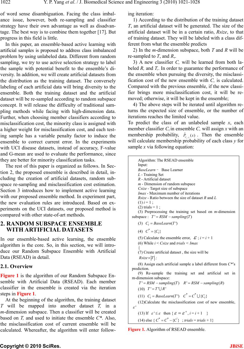

Y. P. Yang et al. / J. Biomedical Science and Engineering 3 (2010) 1021-1028 1022
of word sense disambiguation. Facing the class imbal-
ance issue, however, both re-sampling and classifier
strategy have their own advantage as well as disadvan-
tage. The best way is to combine them together [17]. Bu t
progress in this field is little.
In this paper, an ensemble-based active learning with
artificial samples is proposed to address class imbalanced
problem by using unlabeled data. Different from random
sampling, we try to use active selection strategy to label
the sample with potential benefit to the ensemble’s di-
versity. In add ition , we will create artificial datasets from
the distribution as the training dataset. The conversely
labeling of each artificial data will bring diversity to the
ensemble. Both the training dataset and the artificial
dataset will be re-sampled according to random subspace
concept. It will release the difficulty of traditional sam-
pling methods while facing with high-dimension data.
Further, when choosing member classifiers according to
misclassification cost, the minority class is assigned with
a higher weight for misclassification cost, and each test-
ing sample has a variable penalty factor to induce the
ensemble to correct current error. In the experiments
with UCI disease datasets, instead of accuracy, F-value
and G-mean are used to evaluate the performance, since
they are better for minority classification tasks.
The rest of this paper is organized as follows. In Sec-
tion 2, the proposed ensemble is described in detail, in-
cluding the creation of artificial datasets, random sub-
space re-sampling and misclassification cost estimation.
Section 3 introduces how to implement active learning
with our proposed ensemble method. In experiment part,
the new evaluation rules are introduced. Based on ex-
periments on the UCI datasets, our proposed method is
compared with other state-of-art methods.
2. RANDOM SUBSPACE ENSEMBLE
WITH AR TIFICIAL DATASETS
In our ensemble-based active learning, the ensemble
algorithm is the core. So, in this section, we will intro-
duce our Random Subspace Ensemble with Artificial
Data (RSEAD) in detail.
2.1. Overview
Figure 1 is the algorithm of our Random Subspace En-
semble with Artificial Data (RSEAD). Each member
classifier in the ensemble is created via the iteration
steps in Figure 1.
At the beginning of the algorith m, the training dataset
T will be mapped into another dataset T, in a
m-dimension subspace. Then a classifier will be created
based on T, and used to initiate the ensemble C*. Also,
the misclassification cost of current ensemble will be
calculated. Whereafter, the algorithm will enter follow-
ing iteration:
1) According to th e distribution of the training dataset
T, an artificial dataset will be generated. The size of the
artificial dataset will be in a certain ratio, Rsize, to that
of training dataset. They will be labeled with a class dif-
ferent from what the ensemble predicts
2) In the m-dimension subspace, both T and R will be
re-sampled to T, and R,.
3) A new classifier C, will be learned from both la-
beled R, and T,. In order to guarantee the performance of
the ensemble when pursuing the diversity, the misclassi-
fication cost of the new ensemble with C, is calculated.
Compared with the previous ensemble, if the new classi-
fier brings more misclassification cost, it will be re-
moved; otherwise, it will be kept in the ensemble;
4) The above steps will be iterated until algorithm re-
turns the expected size of ensemble, or the number of
iterations reaches the limited value.
To predict the class of an unlabeled sample x, each
member classifier Ci in ensemble C, will assign x with an
membership probability, ,
ˆ()
i
Cy
Px . Then the ensemble
will calculate membership probability of each class y for
sample x via following equation:
Figure 1. Algorithm of RSEAD ensemble.
Algorithm: The RSEAD ensemble
Input:
BaseLearn– Base Learner
L - Training Set
R - Artificial dataset
m - Dimension of random subspace
Csize - Target size of subspace
Imax - Maximum number of iterations
Rsize - Ratio between the size of dataset R and L
(1) i = 1 ;
(2) trials = 1 ;
(3) Preprocessing the training set based on m-dimension
subspace : '()TRSMsamplingT


(3) (')
i
CBaseLearnT
(4) *{}
i
CC
(5) Calculate the ensemble error,

; i = i + 1
(6) While i < Csize and trials < Imax
{
(7) Create artificial dataset , the size will be
R
size T

;
(8) Assign each artificial sample a lab el different from C*’s
prediction.
(9) Re-sample the training set and artificial set in
m-dimension subspace:
'()TRSMsamplingT

 '()
R
RSMsampling R
(10) '''TTR
(11) (')
i
CBaseLearnT **
{}
i
CC C
(12)Calculate the misclassification cost of new ensemble,
'

(13) If '



then {'


 , i = i + 1 }
(14) else {** ' {}CC C ; trials = trials + 1}

Y. P. Yang et al. / J. Biomedical Science and Engineering 3 (2010) 1021-1028
1023
*,
*
ˆ()
ˆ()
i
i
Cy
CC
y
Px
Px C



(1)
Equation (1) reflects the probability of x belonging to
class y. Therefore, the label with largest membership
probability will be assigned to x:
*ˆ
( )argmax( )
y
yY
Cx Px

 (2)
2.2. Creation and Labeling of Artificial Datasets
The diversity is a critical factor for a successful ensem-
ble [11]. An ensemble will have less diversity if its
member classifiers have the same property. To bring
more diversity, Bagging [19] divides the training set into
several smaller one, while Boosting adjusts the distribu-
tion of the training dataset according to the chosen clas-
sifier [20]. Further, in Random Forest [21], both training
dataset and feature space are divided into smaller ones to
train different classifiers. However, all these methods
depend on the training dataset to induce the diversity.
Therefore, if the training dataset is not big enough, the
diversity will be limited.
In our active learning method, the RSEAD ensemble’s
diversity will be guaranteed in three ways: 1) with active
learning, the large pool of unlabeled data can be sampled
to get good training datasets; 2) besides the training da-
taset, the artificial data are also created for training clas-
sifier; 3) both the original training and the artificial da-
tasets will be re-sampled in subspace to enhance diver-
sity. In this part, we will focus on the creation of artifi-
cial dataset and their labeling.
In our method, the artificial data are created by ran-
domly picking data points from an approximation of the
training dataset distribution. The numeric attributes are
defined according to the mean and the standard deviation
of the training dataset, and generated in Gaussian distri-
bution. For a nominal attribute, its value is based on the
probability of the occurrence of each distinct value in its
domain. The Laplace smoothing is used if a certain no-
minal attribute is absent in the training dataset. Further,
to construct an artificial data, there is a simplifying as-
sumption that the attributes are independent, because it
will cost much time and labeled data to accurately esti-
mate the joint probability distribution of these attributes.
In each iteration shown in Figure 1, the ensemble will
predict the class label for each artificial data x. Firstly,
ensemble will give a membership probability of x be-
longing to certain class y. The zero membership prob-
ability will be replaced by a small non-zero value in case
that it may act as a denominator. Then the artificial data
will be labeled a class that is different from what the
ensembles predict. Therefore, if current ensemble pre-
dicts the probability of x belonging to y is ˆ()
y
P
x, then,
the choice of label for x will be based on '
ˆ()
y
Px:
'ˆ
1/()
ˆ() ˆ
1/()
y
y
y
y
Px
Px Px  (3)
Let us show this labeling method with a two-class
problem. For instance, for an artificial sample x, the en-
semble estimates that it has 20% probability of being a
positive sample and 80% probability of being a negative
one. In other words, the ensemble believes that x is more
likely a negative sample. In our method, to create a new
classifier with more diversity, x will be assigned with a
positive label, and th en used to train a new classifier.
The ensemble often has higher accuracy than single
member classifier if each member classifier is not related
with others. Therefore, our method of labeling artificial
data can reduce the relevancy between classifiers, which
will in turn bring the ensembl e with higher accuracy and
less generalization error.
2.3. Re-Sampling in Subspace
Re-sampling is the popular way to deal with class im-
balance problem. However, most of sampling methods,
like SMOTE, often work in the whole feature space,
which is not efficient in countering high-dimension da-
tasets. In addition, they often try to consider the class
imbalance and the properties of the dataset as a whole.
The data, however, often exhibit characteristics and
properties at a local level, rather than the global level.
Hence, it is important to study the dataset in a reduced
subspace. Although a certain feature subspace may only
lead to a weak classifier, the ensembling of such weak
ones can make a strong classifier [22], since it induces
higher diversity, which is an important condition for a
classifier with good performance.
To this end, we proposed the Random-Subspace-
Mapping Sampling (RSM-sampling) algorithm.
Suppose we have a dataset L, which has a
n-dimension space: |L| = l, 12 { ,,...,}
n
F
FF F. Any data
PL

can be represented as 12 { ,,...,}
n
PPP P, where
i
P is the value of the related feature i
F
in the feature
space F.
If the dimension of each subspace is set to m, m<n, the
number of the likely subspace will be max m
n
kC. When
[/2]mn

, kmax has its biggest value. For our algorithm,
each feature subspace will bring a candidate classifier.
We often choose Cszie< kmax classifiers to construct an
ensemble, since not every candidate classifier will help
enhance the ensemble,s performance.
Before re-sampling, a subspace S should be randomly
selected from the feature space F.
F
mn

.
12
{, ,...,}
m
SSS SF

. Then, in the feature subspace,

Y. P. Yang et al. / J. Biomedical Science and Engineering 3 (2010) 1021-1028 1024
each data PL will be mapped into
12 { ,,...,}
Sss sm
PPP P.
In each iteration step of our algorithm, both the train-
ing dataset L and the artificial dataset R are re-sampled
in chosen sub-space.
2.4. Misclassification Cost Estimation
When pursuing the diversity, the performance of ensem-
ble should be guaranteed too. To address the problem of
class imbalance, the misclassification cost is used to
replace the traditional classification error. A new classi-
fier will be kept in the ensemble if it helps decrease the
misclassification cost; otherwise, it will be removed.
In our algorithm, the minority class is assigned with a
higher weight of misclassification cost than that of the
majority class. Also, each test sample will be assigned
with a penalty factor. If current ensemble makes wrong
decision on it, its penalty factor will be increased; oth-
erwise, its penalty factor will be decreased. In this way,
the ensemble will choose the new classifier that helps to
correct the error of current ensemble. Also, since the
minority samples have more chance to be misclassified,
this penalty factor will bring an ensemble proper for
minority class.
Suppose we have t samples to evaluate the ensemble
based on misclassification cost. Firstly, each sample’s
penalty factor will be initialized as:
11/ 1
i
dtit (4)
The misclassification cost of the ensemble gotten in
k-th iteration can be represented as:
*
1
cos (,())
tk
kikii
i
tyC xd 


 (5)
In Equation (5), yi is the correct class label of testing
sample xi, *()
ki
Cx is the predicted class o f the en semble
for xi. k
i
d is xi,s penalty factor for the k-th iteration.
*
cos (,())
iki
tyC x is the weight of misclassifying a sam-
ple with label yi as class *()
ki
Cx. When*()
iki
y
Cx,
there is*
cos (,())0
iki
tyC x because classification is
correct.
If the misclassification cost in the k-th iteration is less
that that in the (K–1)-th iteration, then newly created
classifier will be kept in ensemble. There, we have the
coefficient of perf o rmanc e enhancing:
ln((1) /) / 2
kkk

  (6)
Each testing sample’s penalty factor will be modified
according to current ensemble’s prediction. If current
ensemble makes correct classification on xi, its penalty
factor 1k
i
d will be decreased to:
1exp( ) kk
ii k
dd a
 (7)
Otherwise, it will be increased to:
1exp( ) kk
ii k
dd a
 (8)
Please note, all samples, new penalty factors will be
normalized as following:
1
11
tk
ki
i
Z
d



11
1
/
kk
iik
ddZ


. (9)
1k
i
d

will be used in the (k + 1)-th iteration.
The design of misclassification cost weigh
*
cos (,())
iki
tyC xand penalty factor1k
i
d will help the
ensemble to pick the classifiers that can better deal with
minority class.
3. ACTIVE LEARNING WITH THE
ENSEMBLE RSEAD
The ensemble with diversity will be used in active
learning for selecting unlabeled data. Like the QBC [23],
our proposed active learning method also chooses the
unlabeled samples that have the biggest prediction dif-
ference among the classifiers in the ense mble. Such pre-
diction difference is often called uncertainty, which is
calculated via margin measure in our algorithm. The
margin is defined as the difference of membership
probability between the samples most likely class and
second most likely class.
*12
ˆˆ
(,) ()()
yy
M
argin CxPxPx (10)
where y1 and y2 are class labels of unlabeled sample x
predicted by ensemble C*. y1 has the highest member-
ship probability for x, while y2 is the second high est one.
Then, the uncertainty can be represented as:
*1
(,) (*, )
UncertaintyCxMargin Cx

 (11)
where the
 is a small value in case margin is 0. The
smaller margin is, the bigger the uncertainty is. For a
two-class task, when12
ˆˆ
() ()
yy
Px Px，the margin will be
0, and x will have the biggest uncertainty,
*
(,)1/UncertaintyCx


4. EXPERIMENTS
To evaluate our method,s effectiveness for medical di-
agnosis, eight disease datasets from the UCI machine
learning repository [24] are used in experiments. In this
section, we will discuss the experiments in detail.
4.1. Evaluation Rule
In a two-class task, a classifier will have four kinds of
prediction results [25] for dataset with N samples, shown
in Table 1. TP and FN responsively mean the number of
correctly and wrongly classified positive samples, while

Y. P. Yang et al. / J. Biomedical Science and Engineering 3 (2010) 1021-1028
1025
TN and FP mean the number of correctly and wrongly
classified negative samples.
The classification accuracy is often calculated as :
Accuracy = (TP+FN)/N. (12)
The accuracy rule, however, is not a good one for im-
balance classification [26], for example, if there are only
1% positive samples but 99% negative samples. Simply
classifying all samples as negative class will bring 99%
accuracy, but misclassified 1% positive samples will
bring enormous cost. Therefore, such 99% accuracy is a
disaster for medical diagnosis.
In our proposed method, F-value [27] defined in Equ-
ation (13) is used to evaluate the classifier for imbalance
class problem.
2
2
(1 )
F value


 

Precision Recall
Precision+Recall (13)
where, Precision = TP/(TP+FN); Recall = TP/(TP+FP).
β measures the importance of Precision vs. Recall. In
our method, β = 1, which means Precision and Recall
is equally important.
In addition, G-Mean [28] is also used in evaluating the
performance of our classifier.
G-mean= PositiveAccuracyAccuracyNegative (14)
where PossitiveAccuracy = Precision, NegativeAccuracy
= TN/(TN+FP). It can be seen that G-mean measure tries
to build a balance between positive class and negative
class.
4.1. Datasets Description
For testing, eight disease datasets from UCI are chosen.
Some basic information about them is summarized in
Table 2, in which P:N means the number of positive
samples via number of negative samples.
4.2. Experiments on the Dimension of Subspaces
As discussed in 2.3, to randomly select a m-dimension
subspace from a n-dimension feature space, the number
of choices will be max m
n
kC. In our algorithm, the m is
recommended as [/2]mn, since it bring the maxim
choice. Even if we choose a Csize < Kmax, bigger value
of kmax means more chance to get good member classifi-
ers.
Based on dataset Breast-w, we test the relation be-
tween the dimension of a subspace and the performance
of a classifier based on F-value. The result is shown in
Figure 2. In this experiment, the Csize of the ensemble
is 30. Since Breast-W has 9 features, m = 1 a nd m = 9 ar e
meaningless to this experiment. So, the dimension of
feature space m will be changed from 2 to 8 in experi-
ment. In Figure 2, F-value will reach its peak when m =
5. The F-value at m = 4 is a little less than m = 5, al-
though they have the same kmax. The reason may be that
5-feature subspace brings more information than
4-feature one. From Figure 2, we can see that if m is too
small, the information in each subspace is too little to
train a good classifier; but if m is too big, there will be
little diversity among different subspace, which is also
bad for the performance of the ensemble. This experi-
ment shows that m = [n/2] is a good setting for dataset
Breast-W.
4.3. Experiment on the Size of Ensemble
In this experiment, we test the relation between the en-
semble’s size and its classification performance. The
Breast-W is still used and t he result is shown in Figure 3.
Table 1. Classification of a two-class problem.
#classified as
positive
#classified as
negative
Total
Positive sampleTP FN TP+FN
Negative sampleFP TN FP+TN
Total TP+FP FN+TN N
Table 2. Summary of experimental UCI disease datasets.
Dataset #features #instances P：N
Colic 22 368 136：232
Sick 30 3772 231：3541
Diabetes 8 768 268:500
SAheart 11 462 160:302
Hepatitis 20 155 32:123
mammograph 5 961 445:516
Breast-W 9 699 241:458
Spect 22 267 55:212
Figure 2. F-value for different dimension of subspace on
Breast-W dataset.

Y. P. Yang et al. / J. Biomedical Science and Engineering 3 (2010) 1021-1028 1026
Figure 3. F-Value for different size of an ensemble on
Breast-W dataset.
In the experiment, the dimension of subspace is fixed
as [/2][9/2] 5mn. Therefore, there will be
5
9126Cchoices of subspaces to train Csize classifiers
for the ensemble. In Figure 3, the F-value increases
quickly when Csize grows from 10 to 30, but the en-
hancement is not big when Csize is changed from 30 to
120. It shows that for dataset Breast-W, 30 subspaces
with 5 dimension s are enough to build a good ensemble.
The additional subspace will contribute little to the di-
versity of ensemble, and there will be no much en-
hancement in performance, though the computation cost
grows much. Therefore, 30 is a trade-off between per-
formance and computation cost for dataset Breast-W.
4.3. Experiment Result
In this experiment, we firstly test the performance of our
proposed RSEAD ensemble algorithm. For comparison,
two state-of-art classification algorithms, Bagging and
Adaboost, are chosen. For fair comparison, C4.5 is used
as base learner, and is configured with the default setting
in Weka [29]. In the evaluation of performance, F-value
and G-mean are used in experiments with 10-fold cross
validation. For RSEAD algorithm, it has a setting with
[/2]mn，k = 30, and Imax = 50.
Shown in Table 3 is the F-value for the minority class
in each dataset, while Ta b le 4 is the G-value for every
whole dataset. For each dataset, the highest value is
marked in bold. For convenience of comparison, the
base learner C4.5 is also used as the reference. In the
tables, Ada represents the Adaboost algorithm.
In Ta bl e 3 and 4., all 3 ensembles have good F-value
and G-mean than C4.5 on eight datasets. Compared with
Bagging and Adaboost, our RSEAD has higher F-value
and G-mean on most of dataset. From Tab le 3, it can be
concluded that RSEAD has the best performance for
minority class on 6 datasets. On dataset mammo g raph ,
the difference between ensembles is not significant. The
reason may be that ratio between the minority and ma-
jority classes is near 4:5, which has a very small class
imbalance. Also, dataset mammograph is defined only
by 5 features, which leaves little room for our random
subspace re-sampling method to enhance the ensemble's
performance. In the evaluation based on G-mean, our
RESEAD wins for all 8 datasets. From Tables 3 and 4, it
can be seen that our ensemble RESEAD has better per-
formance than Bagging and ADABOOST in countering
problem of imbalance class. This advantage comes from
the unique way of creating each member classifier as
well as the misclassification cost based decision in se-
lecting proper classifiers. Compared with Bagging,
Adaboost has better performance, because Adaboost
introduces different cost weight for different misclassi-
fication. It also indirectly proves the correctness of our
misclassification cost estimation.
To further test the performance of our active learning
method with RSEAD ensemble, the Bagging and Ada-
boost are also merged into the active learning architec-
ture for comparison. Single RSEAD is tested further as
reference. Tab le 5 shows how many samples each algo-
rithm needs to get certain F-value on each dataset.
Compared with RSEAD, the active learning methods
need fewer samples to get the same F-value. Among the
three active learning methods, our Active-RSEAD has
significant advantage, which benefits from the design of
RSEAD ensemble.
Table 3. F-vaule for minority class in each dataset.
Dataset C4.5 RSEAD Bagging Ada
Colic 76.54 80.97 79.71 80.03
Sick 87.65 93.23 90.44 91.43
Diabetes 61.4 71.8 67.9 69.8
SAheart 55.3 75.2 67.4 73.1
Hepatitis 52.8 68.4 67.2 68.5
mammograph 79.5 81.2 82.1 83.2
Breast-W 89.7 95.6 92.3 94.0
Spect 73.1 79.76 76.6 77.5
Table 4. G-mean for each dataset.
Dataset C4.5 RSEAD Bagging Ada
Colic 81.5 85.5 83.4 84.51
Sick 91.2 95.8 95.6 95.2
Diabetes 64.3 76.4 71.4 74.3
SAheart 60.4 77.8 72.3 77.5
Hepatitis 58.4 76.3 74.3 73.4
mammograph 88.4 89.4 89.1 89.3
Breast-W 94.3 96.5 95.3 95.4
Spect 82.3 85.6 82.4 83.4

Y. P. Yang et al. / J. Biomedical Science and Engineering 3 (2010) 1021-1028
1027
Table 5. Number of sampling for target F-vlalue.
Dataset RSEAD Active-RSEAD Active-Bagging Active Adaboost Target F-value
Colic 41 23 35 37 85%
Sick 321 134 178 165 93%
Diabetes 245 101 114 106 75%
SAheart 280 123 157 167 60%
Hepatitis 117 45 56 54 95%
mammograph 100 24 35 30 80%
Breast-W 32 36 45 75 95%
Spect 53 38 43 39 75%
5. CONCLUSIONS
To address the problem of imbalance class in medical
diagnosis, an ensemble-based active learning method is
proposed. Our ensemble algorithm, RSEAD, introduces
the subspace sampling method to reduce the complexity
of computation and bring more diversity together with
the creation of artificial datasets. Further, in evaluating
the quality of each classifier candidate based on misclas-
sification cost, the minority class is assigned with a
higher weight for misclassification costs, while each
testing sample has a variable penalty factor to induce the
ensemble to correct current classification error.
In above experiments, eight UCI disease datasets are
chosen. The F-value and G-mean are used instead of
classification accuracy to evaluate the performance of
classifiers. The result shows that our proposed ensemble
method has better performance than others. Moreover, in
active learning experiment, having the same perform-
ance with F-value rule, our method needs fewer samples.
These experiments show that our ensemble-based active
learning method has significant advantage than tradi-
tional methods.
Ensemble-based active learning is a promising method
to counter the problem of class imbalance in medical
diagnosis. But, there are still many issues for further
studying. For example, our method only deals with
two-class tasks, while the real world has many mul-
ti-class tasks. In addition, the noise in a dataset is not
considered in current study. Also, the weighting method
in our method needs further improvement from both
theory and implementation. Therefore, we will focus on
these issues to improve our active-RSEAD method in
following research work.
REFERENCES
[1] Japkowicz, N. and Stephen, S. (2002) The class imbal-
ance problem: A systematic study. Intelligent Data
Analysis, 6(5), 203-231.
[2] Gustavo, E.A., Batista, P.A., Ronaldo, C., et a1. (2004) A
study of the behavior of several methods for balancing
machine learning training data. SIGKDD Explorations,
6(1), 20-29.
[3] Settles, B. (2009) Active Learning Literature Survey.
Computer Sciences Technical Report 1648, University of
Wisconsin-Madison.
[4] Tomek, I. (1976) Two modifications of CNN. IEEE
Transaction on Systems Man and Communications, 6,
769-772.
[5] Hart, P.E. (1968) The condensed nearest neighbor rule.
IEEE Transaction on Information Theory, 14(3), 515-
516.
[6] Laurikkala, J. (2001) Improving identification of difficult
small classes by balancing class distribution. Proceedings
of the 8th Conference on AI in Medicine, Cascais, Portu-
gal, Europe: Artificial Intelligence Medicine, 63-66.
[7] Wilson, D.L. (1972) Asymptotic properties of nearest
neighbor rules using edited data．IEEE Transaction on
Systems, Man and Communications, 2(3), 408-421.
[8] Chawlan, V., Bowyer, K.W. and Hall, L.O. (2002)
SMOTE: Synthetie minority over-sampling technique.
Journal of Aflificial Intelligence Research, 16(1), 321-
357.
[9] Joshi, M., Kumar, V. and Agarwal, R. (2001) Evaluating
boosting algorithms to classify rare classes: Comparison
and improvements. Proceedings of the 1st IEEE Interna-
tional Conference on Data Mining. Washington DC:
IEEE Computer Society, 257-264.
[10] Akbani, R., Kwek, S. and Japkowicz, N. (2004) Applying
support vector machines to imbalanced datasets. Pro-
ceedings of the 15th European Conference on Machines
Learning, Pisa, Italy, 39-50.
[11] Krogh, A. and Vedelsby, J. (1995) Neural network en-
sembles, cross validation and active learning. Advances
in Neural Information Processing Systems, 7, 231-238.
[12] Provost, F. (2000) Machine learning from imbalanced
data sets 101. Invited paper for the AAAI, Workshop on
Imbalanced Data Sets, Menlo Park, CA.
[13] Abe, N. (2003) Invited talk: Sampling approaches to
learning from imbalanced datasets: Active learning, cost
sensitive learning and beyond. ICML-KDD Workshop:
Learning from Imbalanced Data Sets.
[14] Ertekin, S., Huang, J. and Giles, C.L. (2007) Active
learning for class imbalance problem. Proceedings of
Annual International ACM SIGIR Conference Research
and development in information retrieval, Amsterdam,
Netherlands, 823-824.
[15] Ertekin, S., Huang, J., Bottou, L. and Giles, C.L. (2007)
Learning on the border: Active learning in imbalanced

Y. P. Yang et al. / J. Biomedical Science and Engineering 3 (2010) 1021-1028 1028
data classification. Proceedings of the sixteenth ACM
conference on Conference on information and knowledge
management, November 6-8, Lisboa, Portugal, 127-136.
[16] Zhu, J. and Hovy, E. (2007). Active Learning for Word
Sense Disambiguation with Methods for Addressing the
Class Imbalance Problem. In Proc. Joint Conf. Empirical
Methods in Natural Language Processing and Computa-
tional Natural Language Learning, Prague, 783-790.
[17] Chawla, N.V., Lazarevic, A. and Hall, O. (2003) SMOTE-
Boost: improving prediction of the minority class in
boosting: knowledge discovery in databases. Proceeding
of the 7th European Conference on Principles and Prac-
tice of Knowledge Discovery in Databases. Cavtat Du-
brovnik, 107-119.
[18] Veropoulos, K., Campbell, C. and Cristianini, N. (2009)
Con- trolling the sensitivity of support vector machines.
Proc of Intemational Joint Confbrence on AI, 55-60.
[19] Breiman, L. (1996) Bagging predictors. Machine Learn
-ing, 24(2), 123-140.
[20] Abe, N. and Mamitsuka, H. (1998) Query learning strate-
gies using boosting and bagging. Proceedings of the In-
ternational Conference on Machine Learning (ICML),
Morgan Kaufmann, 1-9.
[21] Breiman, L. (2001) Random forests. Machine Learning,
2001, 45(1), 5-32.
[22] Kleinberg, E.M. (1990) Stochastic discrimination. Annals
of Mathematics and Artificial Intelligence, 1(1-4), 207-
239.
[23] Seung, H.S., Opper, M. and Sompolinsky, H. (1992)
Query by committee. In Proceedings of the ACMWork-
shop on Computational Learning Theory, 287-294.
[24] Blake, C., Keogh, E., and Merz, C.J. UCI repository of
machine lea r n i ng database s. http://www.ics.uci.edu
[25] Su, C.T., Chen, L.S. (2006) Knowledge acquisition
through information granulation for imbalanced data.
Expert Systems with applications, 31, 531-541.
[26] Joshi, M. (2002) On evaluating performance of classi-
fiers for rare classes. Proceeding of the 2nd IEEE In-
ternational Conference on Data Mining, Maebishi, Japan,
641-644.
[27] Kotsiantis, S., Kanellopoulos, D., Pintelas, P. (2006)
Handling imbalanced datasets: A review. GESTS Interna-
tional Transactions on Computer Science and Engineer-
ing, 30(1), 25-36.
[28] Guo, H., Viktor, H. (2004) Learning from imbalanced
data sets with boosting and data generation: the Data-
Boost-IM approach. Sigkdd Explorations, 6(1), 30-39.
[29] Witten, I. H., Frank, E. (2005) Data mining-pracitcal
machine learning tools and techniques with JAVA im-
plementations. 2nd Edition, Morgan Kaufmann Publishers.