Engineering, 2013, 5, 303-308
http://dx.doi.org/10.4236/eng.2013.53041 Published Online March 2013 (http://www.scirp.org/journal/eng)
A Study on the Control Technique of Construction
Project Process*
Changming Hu, Shaoping Zhang, Xueyan Wang
College of Civil Engineering, Xi’an University of Architecture & Technology, Xi’an, China
Received January 15, 2013; revised February 16, 2013; accepted February 23, 2013
ABSTRACT
The construction process control of large-scale projects is one of the difficulties and the keys in the owner’s project
management. Based on generalization process index, this paper proposes an approach to construction project process
control. The paper elaborates on the concept and calculation of generalization process index, which, on analysis, pos-
sesses Markov property. Monthly generalization process index is reg arded as a state of Markov chain, an d the transition
between differen t states is realized by computer simulation. Accord ing to the Markov process forecasting mod el and by
means of MATLAB program, the project process forecast is realized, and the completion probability in contract period
is obtained. From practical instances, it is concluded that this approach has good applicability and operability and that
the obtained results can reflect the degree of project risks.
Keywords: Generalization Process Index; Markov Computer Stimulation; Project Process Control
1. Introduction
Large-scale projects are usually highly professional and
independent, with long construction period, complex en-
gineering structure and complex construction technique,
as well as many cooperative building units. The process
management of such projects directly affects the qualities
of the projects and the production of enterprises. At pre-
sent, the large-scale project management organizations of
most Chinese large enterprises usually employ such tra-
ditional methods as comparison of horizontal diagram,
comparison of S-shaped curve process, comparison of
“banana”-shaped curve. As is indicated by practice, with
the methods above, the project management is strict and
inflexible, which disadvantages the contractor and in-
creases the owner’s management load. Therefore, with
the premise of set quality and schedule, a more applica-
ble project process control approach ought to be sought,
in order to overcome the defects of the traditional meth-
ods in satisfying practical engineering needs, and to
guarantee management at a higher level.
Process control model based on generalization process
index can provide a new method for schedule control. By
this method the owner can grasp overall progress macro-
scopically and know the risk of engineering project. Its
guidelines are as follows: first, the con cept of generaliza-
tion process index is to put forward; second, the gener-
alization process index, on analysis, possesses Markov
property; third, a Markov stimulated process control
model, based on generalization process index, is estab-
lished; therefore, the completion probability in contract
period is obtained.
2. Concept and Calculation of
Generalization Process I n de x
2.1. Concept of Generalization Process Index
Generalization process index means the sum of the per-
centages of the completed quantities (p lan or actual) of a
project’s separated parts that account for the total quanti-
ties at a specified time, noted as GPI (generalization
process index). If the quantities are plan quantities, the
generalization process index is called plan generalization
process index; if the quantities are actual quantities, ac-
tual generalization process index [1,2].
1
GPI TPA
ni
i
PA


Type: i—the plan or actual completed quantities of
a project’s separated parts at a specified time;
PA
TPA—total quantities of a project;
n—sum of total process at a specified time.
2.2. Calculation of Generalization Process Index
[3]
GPI has been widely used in Baosteel technological
*Foundation item: Xi’an social science plan ning project issue (11J058).
C
opyright © 2013 SciRes. ENG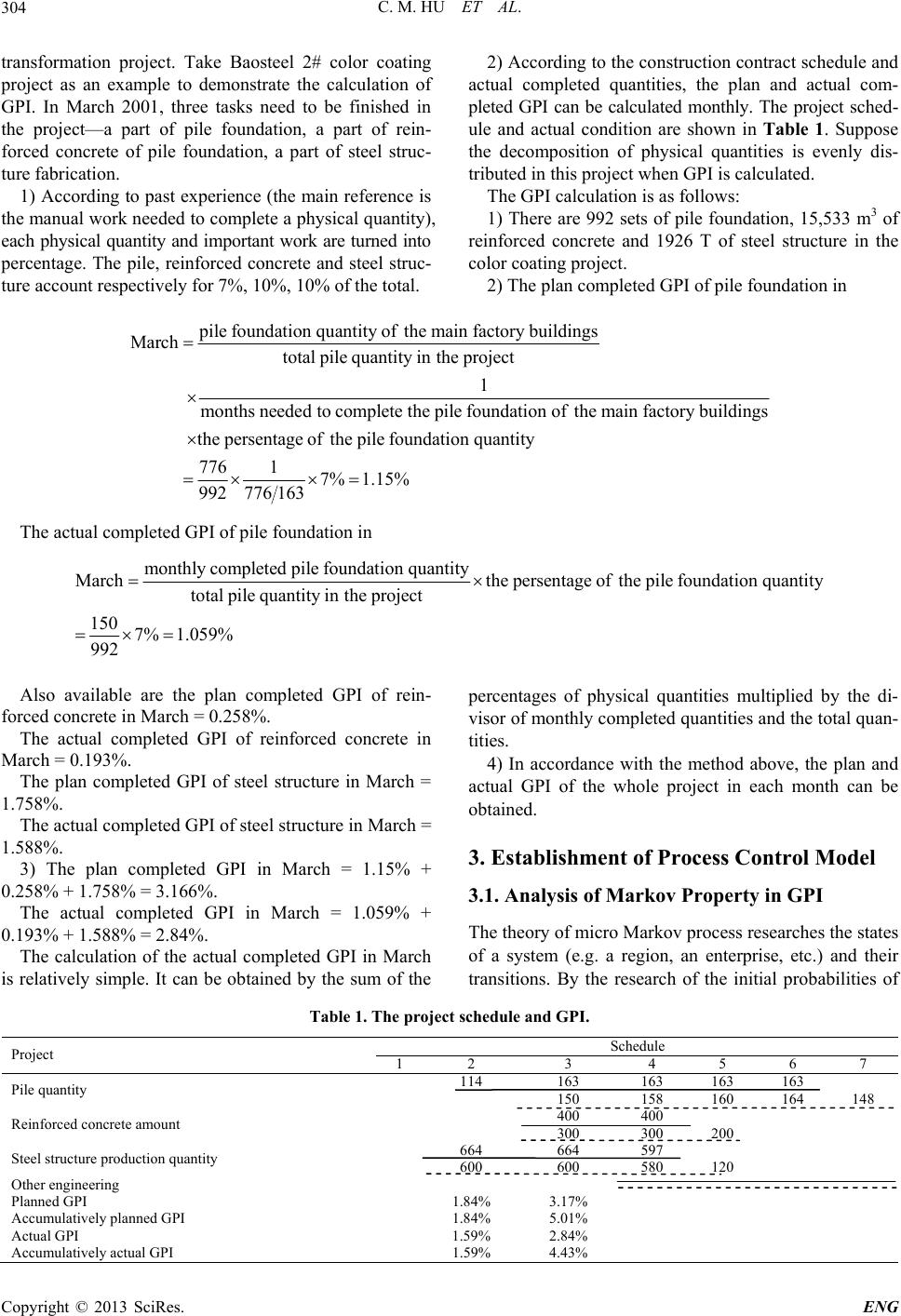

C. M. HU ET AL. 304
transformation project. Take Baosteel 2# color coating
project as an example to demonstrate the calculation of
GPI. In March 2001, three tasks need to be finished in
the project—a part of pile foundation, a part of rein-
forced concrete of pile foundation, a part of steel struc-
ture fabrication.
1) According to past experience (the main reference is
the manual work needed to complete a physical quan tity),
each physical quantity and important work are turned into
percentage. The pile, reinforced concrete and steel struc-
ture account respectively for 7% , 10%, 10% of the total.
2) According to the construction contract schedule and
actual completed quantities, the plan and actual com-
pleted GPI can be calculated monthly. The project sched-
ule and actual condition are shown in Table 1. Suppose
the decomposition of physical quantities is evenly dis-
tributed in this project when GPI is calculated.
The GPI calculation is as follows:
1) There are 992 sets of pile foundation, 15,533 m3 of
reinforced concrete and 1926 T of steel structure in the
color coating project.
2) The plan completed GPI of pile foundation in
pilefoundation quantityofthemainfactorybuildings
March total pile quantityinthe project
1
months needed tocomplete the pilefoundation ofthe main factory buildings
the persentage ofthe pilefoundation quantity
776 1
992 77



 7% 1.15%
6 163
The actual completed GPI of pile foundation in
monthlycompleted pilefoundation quantity
Marchthe persentageofthe pilefoundation quantity
total pile quantity inthe project
150 7% 1.059%
992


Also available are the plan completed GPI of rein-
forced concrete in March = 0.258%.
The actual completed GPI of reinforced concrete in
March = 0.193%.
The plan completed GPI of steel structure in March =
1.758%.
The actual completed GPI of steel structure in March =
1.588%.
3) The plan completed GPI in March = 1.15% +
0.258% + 1.758% = 3.166%.
The actual completed GPI in March = 1.059% +
0.193% + 1.588% = 2.84%.
The calculation of the actual completed GPI in March
is relatively simple. It can be obtained by the sum of the
percentages of physical quantities multiplied by the di-
visor of monthly completed quantities and the total quan-
tities.
4) In accordance with the method above, the plan and
actual GPI of the whole project in each month can be
obtained.
3. Establishment of Process Control Model
3.1. Analysis of Markov Property in GPI
The theory of micro Markov process researches the states
of a system (e.g. a region, an enterprise, etc.) and their
transitions. By the research of the initial probabilities of
Table 1. The project schedule and GPI.
Schedule
Project 1 2 3 4 5 6 7
114 163 163 163 163
Pile quantity 150 158 160 164 148
400 400
Reinforced concrete a mount 300 300 200
664 664 597
Steel structure production quantity 600 600 580 120
Other engineering
Planned GPI 1.84% 3.17%
Accumulatively planned GPI 1.84% 5.01%
Actual GPI 1.59% 2.84%
Accumulatively actual GPI 1.59% 4.43%

C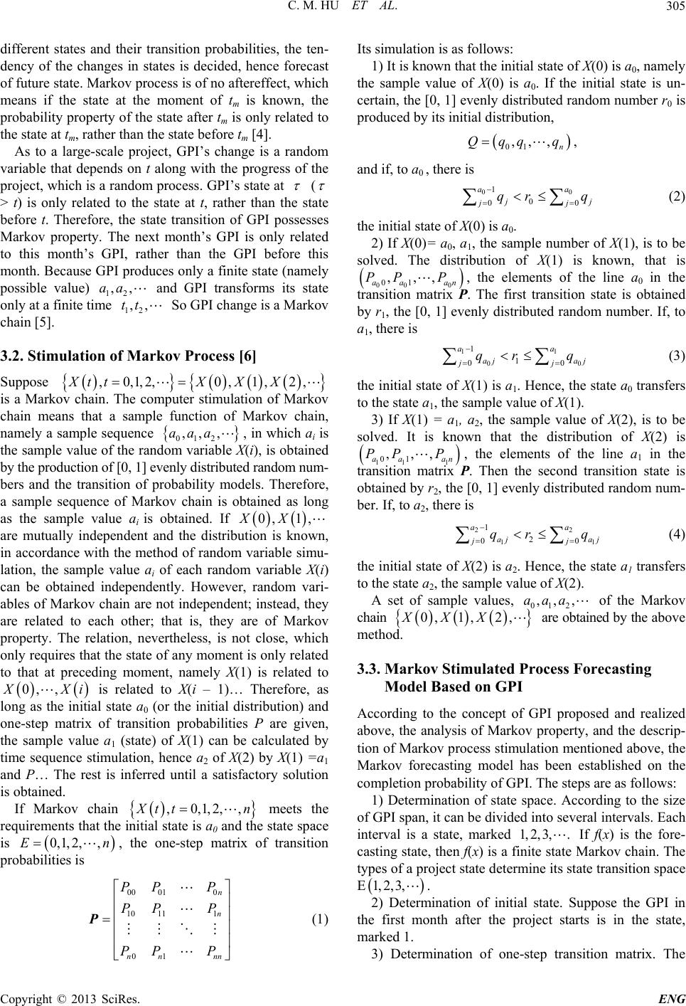. M. HU ET AL. 305
different states and their transition probabilities, the ten-
dency of the changes in states is decided, hence forecast
of future state. Markov process is of no aftereffect, which
means if the state at the moment of tm is known, the
probability property of the state after tm is only related to
the state at tm, rather than the state before tm [4].
As to a large-scale project, GPI’s change is a random
variable that depends on t along with the progress of the
project, which is a random process. GPI’s state at

(

> t) is only related to the state at t, rather than the state
before t. Therefore, the state transition of GPI possesses
Markov property. The next month’s GPI is only related
to this month’s GPI, rather than the GPI before this
month. Because GPI produces only a finite state (namely
possible value) 12 and GPI transforms its state
only at a finite time So GPI change is a Mar kov
chain [5].
,,aa
12
,,tt
3.2. Stimulation of Markov Process [6]
Suppose
   

 
,0,1,2,0,1,2,Xt tXXX

012
,,,aaa



is a Markov chain. The computer stimulation of Markov
chain means that a sample function of Markov chain,
namely a sample sequence , in which ai is
the sample value of the random variable X(i), is obtained
by the production of [0, 1] evenly distribut ed random num-
bers and the transition of probability models. Therefore,
a sample sequence of Markov chain is obtained as long
as the sample value ai is obtained. If


0, 1,XX

,
are mutually independent and the distribution is known,
in accordance with the method of random variable simu-
lation, the sample value ai of each random variable X(i)
can be obtained independently. However, random vari-
ables of Markov chain are not independent; instead, they
are related to each other; that is, they are of Markov
property. The relation, nevertheless, is not close, which
only requires that the state of any moment is only related
to that at preceding moment, namely X(1) is related to

0,
X
Xi is related to X(i – 1)… Therefore, as
long as the initial state a0 (or the initial distribution) and
one-step matrix of transition probabilities P are given,
the sample value a1 (state) of X(1) can be calculated by
time sequence stimulation, hence a2 of X(2) by X(1) =a1
and P… The rest is inferred until a satisfactory solution
is obtained.
If Markov chain
 
,0,1,2,,
X
tt n

n
meets the
requirements that the initial state is a0 and the state space
is , the one-step matrix of transition
probabilities is

0,1,2, ,E
00 010
10 111
01
n
n
nn nn
PP P
PP P
PP P






P




Its simulation is as follows:
1) It is known that the initial state of X(0) is a0, namely
the sample value of X(0) is a0. If the initial state is un-
certain, the [0, 1] evenly distributed random number r0 is
produced by its initial distribution,


01
,,,
n
Qqq q,
and if, to a0 , there is
0
1
0
0
a0
0
a
j
j
j
qr q




j
(2)
the initial state of X(0) is a0.
2) If X(0 )= a0, a1, the sample number of X(1), is to be
solved. The distribution of X(1) is known, that is


,,,
aa an
PP P
000
01 , the elements of the line a0 in the
transition matrix P. The first transition state is obtained
by r1, the [0, 1] evenly distributed random number. If, to
a1, there is
1
0
1
1
0
a
aj aj
j
qr q




1
0
0
a
j
(3)
the initial state of X(1) is a1. Hence, the state a0 transfer s
to the state a1, the sample value of X(1).
3) If X(1) = a1, a2, the sample value of X(2), is to be
solved. It is known that the distribution of X(2) is


,,,
aa an
PP P
11 1
01 , the elements of the line a1 in the
transition matrix P. Then the second transition state is
obtained by r2, the [0, 1] evenly distributed random num-
ber. If, to a2, there is
2
1
1
2
0
a
aj aj
j
qrq




2
1
0
a
j
(4)
the initial state of X(2) is a2. Hence, the state a1 transfer s
to the state a2, the sample value of X(2).
A set of sample values, of the Markov
chain 012
,,,aaa








0, 1,2,XXX are obtained b y the a bo ve
method.
3.3. Markov Stimulated Process Forecasting
Model Based on GPI
According to the concept of GPI proposed and realized
above, the analysis of Markov property, and the descrip-
tion of Markov process stimulation mentioned above, the
Markov forecasting model has been established on the
completion probability o f GPI. The steps are as follows:
1) Determination of state space. According to the size
of GPI span, it can be divided into several intervals. Each
interval is a state, marked If f(x) is the fore-
casting state, then f(x) is a finite state Markov chain. The
types of a project state determine its state t ran sition space
E
1, 2, 3,.


1, 2, 3,.
2) Determination of initial state. Suppose the GPI in
the first month after the project starts is in the state,
marked 1.


(1)
3) Determination of one-step transition matrix. The

C. M. HU ET AL. 306
supervisors and the experts of construction unit, as well
as the engineers gathered by the owner discuss the one-
step transition matrix, which may be modified on a small
scale in the following practice.
4) Prediction of monthly GPI. The GPI and the state
transition matrix in on e month are known; the GPI in the
next month can be predicted.
If the state in the first month 1 is known, the
state in the second month 2is to be solved. According
to the above method of Markov simulation, 2 is to be
determined. The GPI in this month, based on 2 in the
state interval
1a
arr


1, ii
bb
, can be determined with linear in-
terpolation. The GPI in this month iii
is obtained by the production of [0, 1] evenly distributed
random number r. If the GPI in this month is known, the
GPI in the next month can be predicted by the actual GPI.
If the GPI in this month is unknown, the GPI in the next
month can be predicted by the predicted GPI of this
month. The steps are recurred until the completion of
construction.

11
b

Sb b r
5) Determination of completed period. The monthly
GPIs obtained by the above GPI forecasting method are
accumulated. When the accumulated GPI H is not less
than 100%, the construction is completed. According to
the formula, day = (n – 1) + (H – 100)/S, the project
completion period can be obtained.
6) Completion probability in contract period. Accord-
ing to the predetermined number N, after simulation the
number Z is calculated, which indicates the completion
period is not more than the contract period. The comple-
tion probability in the contract period is Z/N. The com-
pletion probability can reflect the project risk in gen-
eral.
By Markov chain stimulation, the forecasting model of
completion probability in contract period based on GPI
can be obtained, which is illustrated in Figure 1.
Identifiers:
m: repeated simulation times day: completion period;
P(I, J): transition probabilities (I, J = 1, 2 ,3, 4, 5);
A: state matrix; T: contract completion period;
N: default maximum completion period;
S: monthly GPI; H: accumulated GPI;
p: completion probability in contract period.
4. Project Application
One steel enterprise is planning to construct a blast fur-
nace of 4350 m3 in order to optimize the industrial struc-
ture and improve economic benefit. This project has been
concluded into the national comprehensive programs.
The project is designed to produce 3.5 million tons of
molten iron, 1.153 million tons of granulating slag. Since
it is a large-scale project, construction enterprise divides
the whole into three sections. One certain Co. Ltd. has
I nput : A, P, m , N,D
K＝1 m
n＝1 N
i=A(n)
r=rand
G=0
j＝1 6
G= G+ p (i,j )
G－p(I,j)<r<=G
r=rand
S=j-1+r,
H=S+H
H> =100%
da y=n - 1+( H-1)/S
D(k)=day
B=D<T
Z= sum(B)
p=Z/N
end
H=0,S=0
n<T
i=j
N
Y
N
Y
N
Y
Output:p
Figure 1. Block diagram of Markov chain stimulation mo-
el. d

C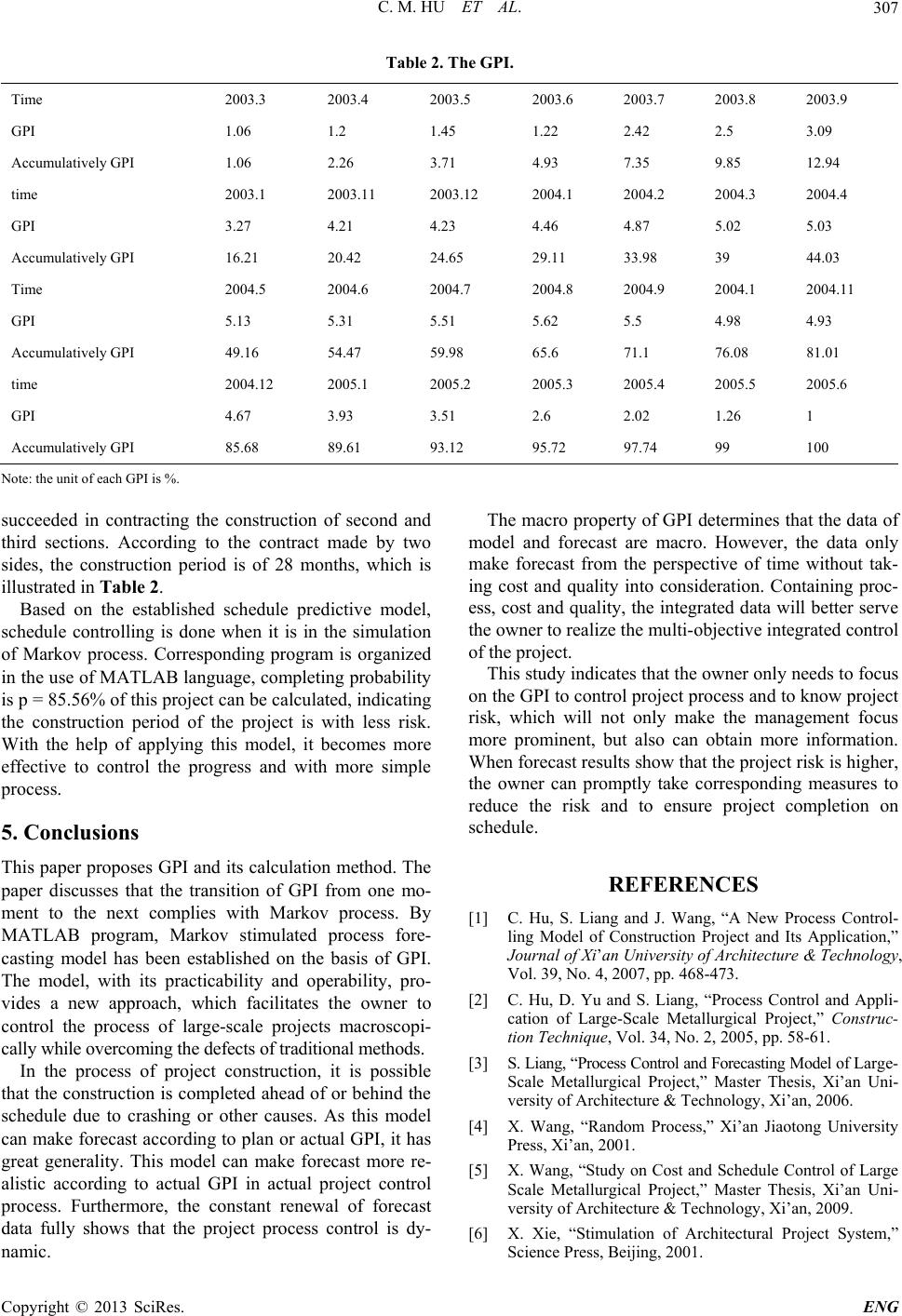. M. HU ET AL. 307
Table 2. The GPI.
Time 2003.3 2003.4 2003.5 2003.6 2003.7 2003.8 2003.9
GPI 1.06 1.2 1.45 1.22 2.42 2.5 3.09
Accumulatively GPI 1.06 2.26 3.71 4.93 7.35 9.85 12.94
time 2003.1 2003.11 2003.12 2004.1 2004.2 2004.3 2004.4
GPI 3.27 4.21 4.23 4.46 4.87 5.02 5.03
Accumulatively GPI 16.21 20.42 24.65 29.11 33.98 39 44.03
Time 2004.5 2004.6 2004.7 2004.8 2004.9 2004.1 2004.11
GPI 5.13 5.31 5.51 5.62 5.5 4.98 4.93
Accumulatively GPI 49.16 54.47 59.98 65.6 71.1 76.08 81.01
time 2004.12 2005.1 2005.2 2005.3 2005.4 2005.5 2005.6
GPI 4.67 3.93 3.51 2.6 2.02 1.26 1
Accumulatively GPI 85.68 89.61 93.12 95.72 97.74 99 100
Note: the unit of each GPI is %.
succeeded in contracting the construction of second and
third sections. According to the contract made by two
sides, the construction period is of 28 months, which is
illustrated in Table 2.
Based on the established schedule predictive model,
schedule controlling is done when it is in the simulation
of Markov process. Corresponding program is organized
in the use of MATLAB language, completin g probability
is p = 85.56% of this project can be calculated, indicating
the construction period of the project is with less risk.
With the help of applying this model, it becomes more
effective to control the progress and with more simple
process.
5. Conclusions
This paper proposes GPI and its calculation method. The
paper discusses that the transition of GPI from one mo-
ment to the next complies with Markov process. By
MATLAB program, Markov stimulated process fore-
casting model has been established on the basis of GPI.
The model, with its practicability and operability, pro-
vides a new approach, which facilitates the owner to
control the process of large-scale projects macroscopi-
cally while overcomi ng the defects of t raditional methods.
In the process of project construction, it is possible
that the construc tion is completed ahead of or behind the
schedule due to crashing or other causes. As this model
can make forecast according to plan or actual GPI, it has
great generality. This model can make forecast more re-
alistic according to actual GPI in actual project control
process. Furthermore, the constant renewal of forecast
data fully shows that the project process control is dy-
namic.
The macro property of GPI determin es that the data of
model and forecast are macro. However, the data only
make forecast from the perspective of time without tak-
ing cost and quality into consideration. Containing proc-
ess, cost and quality, the integrated data will better serve
the owner to realize the multi-o bjective integrated control
of the project.
This study indicates that the own er only need s to focus
on the GPI to contro l project process and to know project
risk, which will not only make the management focus
more prominent, but also can obtain more information.
When forecast results show that the project risk is higher,
the owner can promptly take corresponding measures to
reduce the risk and to ensure project completion on
schedule.
REFERENCES
[1] C. Hu, S. Liang and J. Wang, “A New Process Control-
ling Model of Construction Project and Its Application,”
Journal of Xi’an University of Architecture & Technology,
Vol. 39, No. 4, 2007, pp. 468-473.
[2] C. Hu, D. Yu and S. Liang, “Process Control and Appli-
cation of Large-Scale Metallurgical Project,” Construc-
tion Technique, Vol. 34, No. 2, 2005, pp. 58-61.
[3] S. Liang, “Process Control and Forecasting Model of L a r g e -
Scale Metallurgical Project,” Master Thesis, Xi’an Uni-
versity of Architecture & Technology, Xi’an, 2006.
[4] X. Wang, “Random Process,” Xi’an Jiaotong University
Press, Xi’an, 2001.
[5] X. Wang, “Study on Cost and Schedule Control of Large
Scale Metallurgical Project,” Master Thesis, Xi’an Uni-
versity of Architecture & Technology, Xi’an, 2009.
[6] X. Xie, “Stimulation of Architectural Project System,”
Science Press, Beijing, 2001.

C. M. HU ET AL. 308
Appendix: MATLAB Program
a=input('a=');
P=input('P=');
T=length(a);
b=zeros(1,10);
A=[a,b];
N=length(A);
m=5000;
D=zeros(1,m);
for k=1:m
H=0;S=0;
for n=1:N
if n<T
i=A(n);
else
i=j;
end
r=rand;
G=0;
for j=1:6
G=G+P(i,j);
if G-P(i,j)<r&r<=G
r=rand;
S=(j-1+r)/100;
H=S+H;
break;
end
end
if H>1
day=n-1+(H-1)/S;
D(k)=day;
break;
end
end
end
B=D<T;
p=sum(B)/m;
display(p);