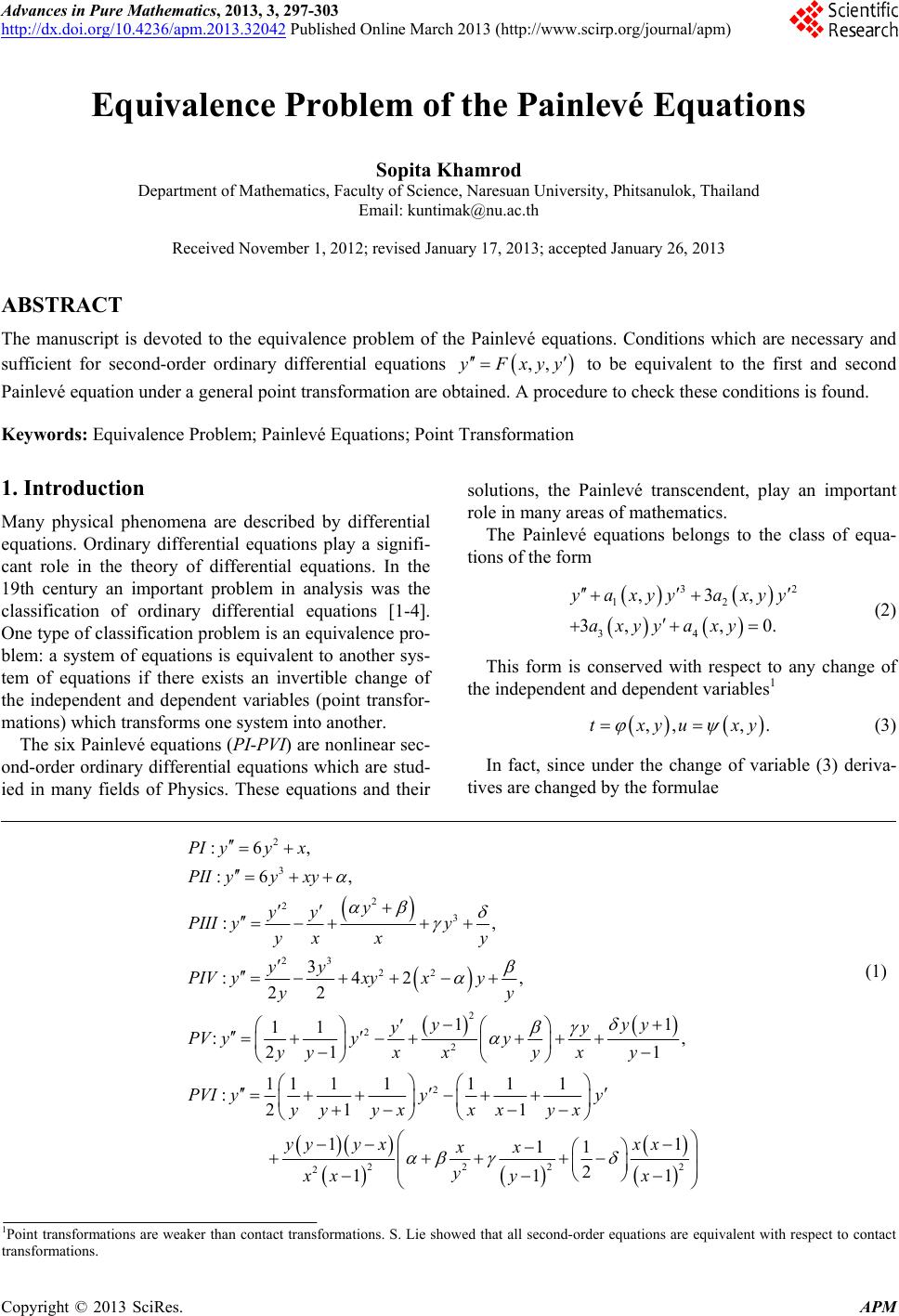
 Advances in Pure Mathematics, 2013, 3, 297-303 http://dx.doi.org/10.4236/apm.2013.32042 Published Online March 2013 (http://www.scirp.org/journal/apm) Equivalence Problem of the Painlevé Equations Sopita Khamrod Department of Mathematics, Faculty of Science, Naresuan University, Phitsanulok, Thailand Email: kuntimak@nu.ac.th Received November 1, 2012; revised January 17, 2013; accepted January 26, 2013 ABSTRACT The manuscript is devoted to the equivalence problem of the Painlevé equations. Conditions which are necessary and sufficient for second-order ordinary differential equations ,, Fxyy to be equivalent to the first and second Painlevé equation under a general point transformation are obtained. A procedure to check these conditions is found. Keywords: Equivalence Problem; Painlevé Equations; Point Transformation 1. Introduction Many physical phenomena are described by differential equations. Ordinary differential equations play a signifi- cant role in the theory of differential equations. In the 19th century an important problem in analysis was the classification of ordinary differential equations [1-4]. One type of classification problem is an equivalence pro- blem: a system of equations is equivalent to another sys- tem of equations if there exists an invertible change of the independent and dependent variables (point transfor- mations) which transforms one system into another. The six Painlevé equations (PI-PVI) are nonlinear sec- ond-order ordinary differential equations which are stud- ied in many fields of Physics. These equations and their solutions, the Painlevé transcendent, play an important role in many areas of mathematics. The Painlevé equations belongs to the class of equa- tions of the form 32 12 34 ,3, 3,, 0. yaxy yaxy y axyy axy (2) This form is conserved with respect to any change of the independent and dependent variables1 ,, ,txyuxy . (3) In fact, since under the change of variable (3) deriva- tives are changed by the formulae 2 3 2 2 3 23 22 2 2 2 2 : 6, : 6, : , 3 : 42, 22 11 11 : , 21 1 11111 1 : 21 PI yyx PII yyxy y yy y y yx xy yy yxy xy yy yyy yy y yy yyxy xy x PVI yy yy yxxx PIII PIV PV (1) 222 2 2 1 1 11 11 2 111 y yx yyyxxx xx y xxy x 1Point transformations are weaker than contact transformations. S. Lie showed that all second-order equations are equivalent with respect to contact transformations. C opyright © 2013 SciRes. APM 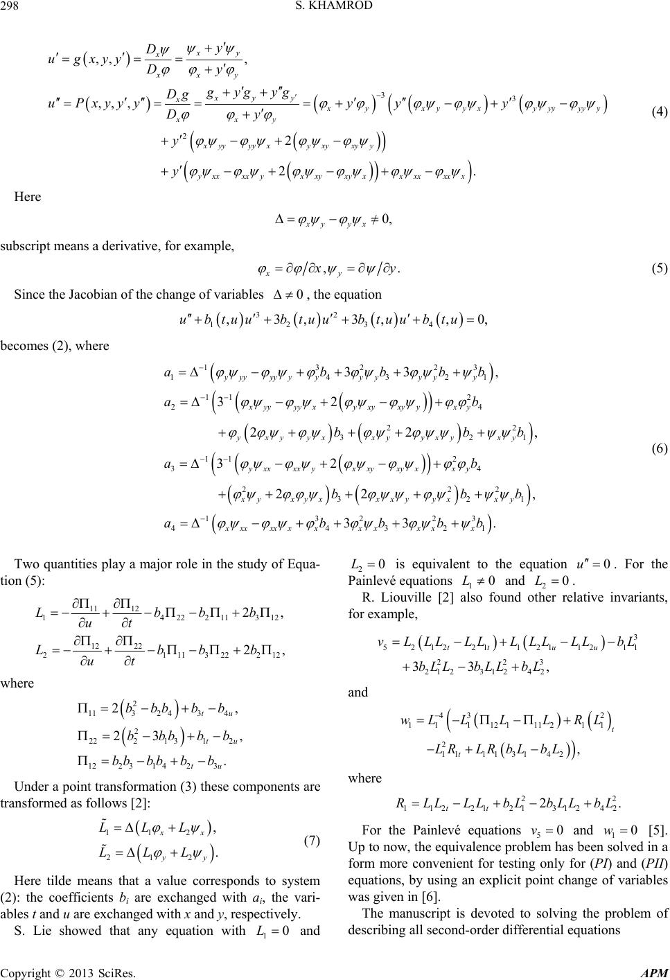 S. KHAMROD 298 33 2 ,, , ,, , 2 xy x xxy xy y x yx yy xy xxy xyy yyxyxyxyy y D ugxyyDy gygyg Dg uPxyyyy yy Dy y yyyy y 2. yxx xxyxxy xyxxxx xxx y 0, yx (4) Here xy subscript means a derivative, for example, , xy y. 0 (5) Since the Jacobian of the change of variables , the equation 4 ,0,b tu 23 1 2 4 22 321 4 , , y y xy y bb ab b ab 2 21 23 1 3. , xy x bb bb 32 123 ,3,3,ub tuubtuubtuu becomes (2), where 132 1 432 11 2 11 2 3 22 3 33 32 22 32 22 yyy yyy yyyyy xyy yyxyxyxyyx yxy yxxyyxy yxxxxyxxy xyxx xyxyxxxy yx abb bb b 13 2 4 432 3 xx x xxxxxxxx ab b (6) Two quantities play a major role in the study of Equa- tion (5): 11 12 14 222 12 22 21 113 Lb ut Lb ut 113 12 222 12 2, 2, bb bb 3 4 31 2 23 . , , tu tu tu b bb bbb b b 112 212 , . xx yy L L 10L where 2 1132 4 2 222 1 12231 4 2 23 bb bb bb bb Under a point transformation (3) these components are transformed as follows [2]: LL LL (7) Here tilde means that a value corresponds to system (2): the coefficients bi are exchanged with ai, the vari- ables t and u are exchanged with x and y, respectively. S. Lie showed that any equation with and 20L is equivalent to the equation u. For the Painlevé equations 0 0L1 and . 2 R. Liouville [2] also found other relative invariants, for example, 0L 3 5212 21121 1211 223 21 23124 2 33 , tt uu vLLLLL LLLLLbL bLLbLL bL and 43 2 11112111211 2 1111 3142 , t t wLLLL RL LRLR bLbL 22 112 212131242 2. tt RLL LLbLbLLbL 0v0w where For the Painlevé equations 5 and 1 [5]. Up to now, the equivalence problem has been solved in a form more convenient for testing only for (PI) and (PII) equations, by using an explicit point change of variables was given in [6]. The manuscript is devoted to solving the problem of describing all second-order differential equations Copyright © 2013 SciRes. APM 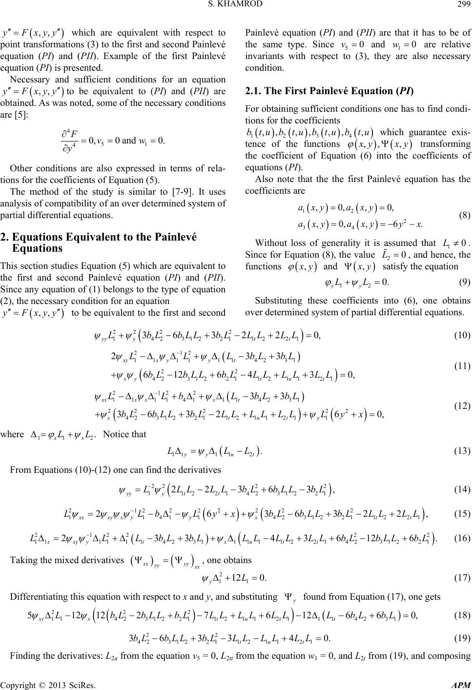 S. KHAMROD 299 ,, Fxyy ,, which are equivalent with respect to point transformations (3) to the first and second Painlevé equation (PI) and (PII). Example of the first Painlevé equation (PI) is presented. Necessary and sufficient conditions for an equation Fxyy to be equivalent to (PI) and (PII) are obtained. As was noted, some of the necessary conditions are [5]: 4 40, F y 51 0 and0.vw ,, Other conditions are also expressed in terms of rela- tions for the coefficients of Equation (5). The method of the study is similar to [7-9]. It uses analysis of compatibility of an over determined system of partial differential equations. 2. Equations Equivalent to the Painlevé Equations This section studies Equation (5) which are equivalent to the first and second Painlevé equation (PI) and (PII). Since any equation of (1) belongs to the type of equation (2), the necessary condition for an equation Fxyy 0 to be equivalent to the first and second Painlevé equation (PI) and (PII) are that it has to be of the same type. Since 5 v and 1 are relative invariants with respect to (3), they are also necessary condition. 0w 2.1. The First Painlevé Equation (PI) For obtaining sufficient conditions one has to find condi- tions for the coefficients 4 ,, ,,,, ,btubtu btu b tu 123 which guarantee exis- tence of the functions ,, , yxy transforming the coefficient of Equation (6) into the coefficients of equations (PI). Also note that the the first Painlevé equation has the coefficients are 12 2 34 ,0,,0, ,0,,6 . axyaxy axyaxyyx 0L (8) Without loss of generality it is assumed that 1 . Since for Equation (8), the value 2, and hence, the functions 0L , , y and y 12 0. yy LL satisfy the equation (9) Substituting these coefficients into (6), one obtains over determined system of partial differential equations. 22 22 142312211221 363220, yt t LbLbLLbLLLLL yy (10) 212 11111142 31 22 42312211 21121 233 612 643 0, xyxyyt xyt ut LLLbLbL bLbLLbLLLL LLL (11) 2122 1111411142 31 22 222 42312211 2112 11 33 36 3260, xxx xxt xtuty LLbLbLbL bLbLLbLLLL LL LLyx .L (12) where 11x L2x Notice that 11112. yy ut LLL 222 2 112214231221 2236 3, yyy tt LLLLLbLbLLbL (13) From Equations (10)-(12) one can find the derivatives (14) 21222222 2 11411 42312211221 2636322, yyxtt LLbLyxbLbLLbLLLLL xxxyx (15) 21 LL 22 22 11111231111122 14231221 3436126. xxyyxu tt LbLbLLLLLLLbLbLLbL yy 1 4 23 t xx yy (16) Taking the mixed derivatives x 2 11 12 0. yL , one obtains (17) Differentiating this equation with respect to x and y, and substituting found from Equation (17), one gets 222 1142 312211211211142 31 5121227 612660, xyxt utt LbLbLLbLLLLLLLLbLbL 22 42312211 21121 36334 0. tut bLbLLbLLLL LL L (18) (19) Finding the derivatives: L2u from the equation v5 = 0, L2tt from the equation w1 = 0, and L2t from (19), and composing Copyright © 2013 SciRes. APM 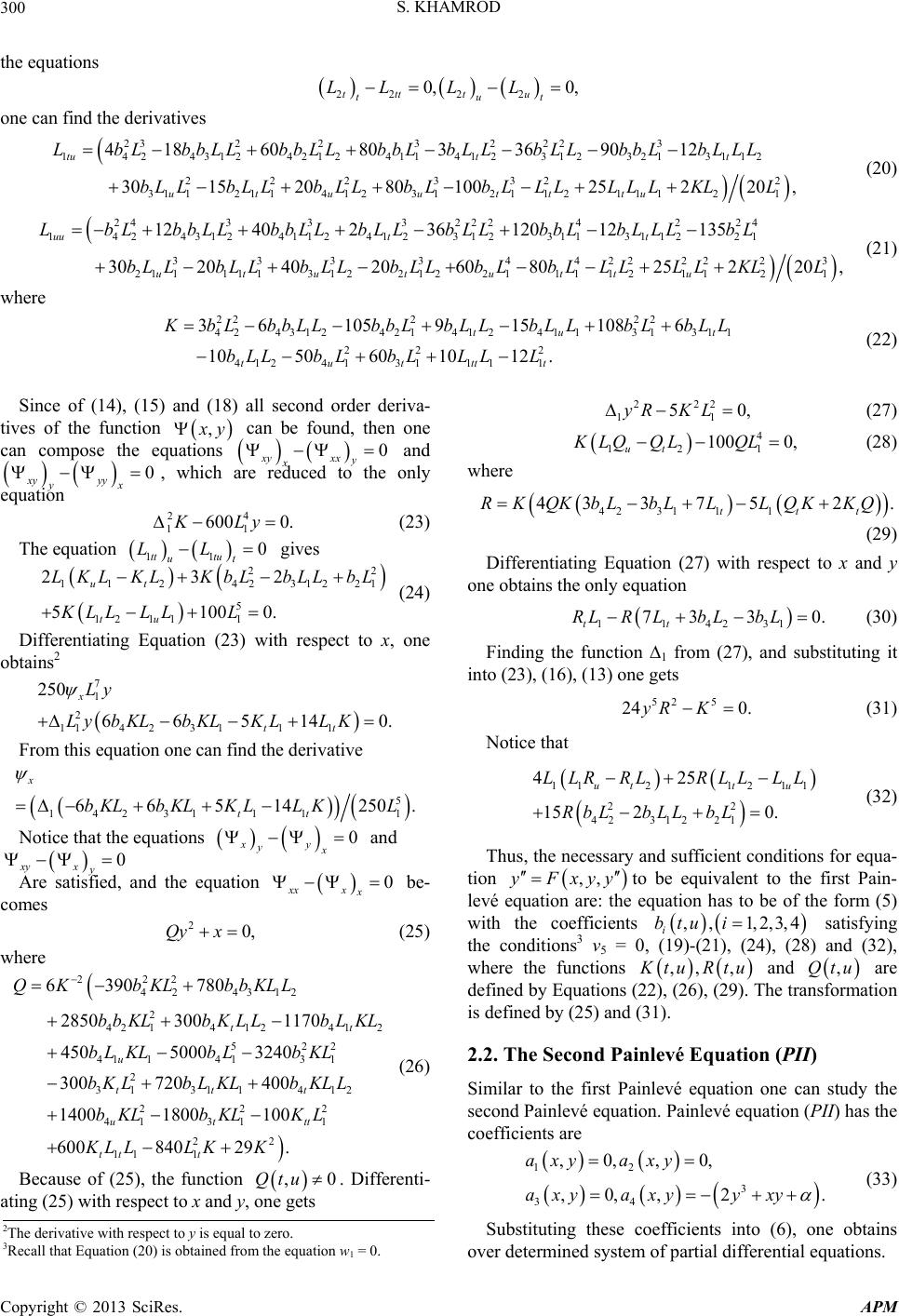 S. KHAMROD 300 the equations 2 2 0, t u t L 22 0, ttt tu LL L one can find the derivatives 232232 223 14243124212411412312321 222 332 31121 14123121121 11 4 1860803369012 30152080 100252 tu utu utttu LbLbbLLbbLLbbLbLLbLLbbL bLLbL LbLLbLbLLLL LLK 3112 2 2 1 20 , tt bLLL L L (20) 2433322242 1424312411241231231131122 3333442222 21 11113 1221221111211 1240236120 12135 3020402060 80252 uut t utu tuttu LbLbbLLbbLLbL Lb LLbbLbL LLb bLLbLLb LLbLLbLbLLLLL 24 1 23 2 1 20 , L KL L 22 31311 6t (21) where 22 2 424312421412411 22 2 4124 1311 11 3 6105915108 1050601012. tu tutttt bL bbLLbbLbLLbLLb bLLbLbLLL L L bLL , (22) Since of (14), (15) and (18) all second order deriva- tives of the function y can be found, then one can compose the equations xy 0 0 24 11 600 0.KLy 11 0 tu LL 22 31221 2 00. bLL bL 1 140. tt LK xx y x and xy yx , which are reduced to the only equation yy (23) The equation gives tt LKLKL ut 11 2 42 5 12 111 23 510 ut tu KbL KLL LLL (24) Differentiating Equation (23) with respect to x, one obtains2 7 1 2 1142311 250 665 xLy Ly bKLbKLKL From this equation one can find the derivative 5 1 1 250 .K L 14 231 1 665 14 x tt bKLbKLKLL Notice that the equations 0 xy x y 0 xx 20,Qy x 12 412 522 3 1 412 2 1 170 tt t tt L b LKL bKL b KLL KL ,0u 222 11 50,yR KL and 0 xyx y Are satisfied, and the equation be- comes xx (25) where 222 42 43 2 42141 2 41 141 2 31 311 22 41 31 22 11 1 6 390780 2850 3001 45050003240 300 720400 14001800 100 60084029 . u tt ut tt t QKbKL bbKL b bKLbKL L bL KLbL bKLbL KL bKL bKL KL LL KK Qt (26) Because of (25), the function . Differenti- ating (25) with respect to x and y, one gets (27) 4 12 1 100 0, ut KLQQLQL (28) where 42 3111 4337 52 ttt RKQKbLbLLLQK KQ . (29) Differentiating Equation (27) with respect to x and y one obtains the only equation 114231 73 30. tt RLR LbLbL 52 5 24 0.yR K (30) Finding the function ∆1 from (27), and substituting it into (23), (16), (13) one gets (31) Notice that 11212 11 22 4231221 425 15 20. utt u LLR RLRLL LL RbLbLLbL (32) Thus, the necessary and sufficient conditions for equa- tion ,, Fxyy to be equivalent to the first Pain- levé equation are: the equation has to be of the form (5) with the coefficients ,, 1,2,3,4btu i i satisfying the conditions3 v5 = 0, (19)-(21), (24), (28) and (32), where the functions ,, , tuRtu and ,Qtu are defined by Equations (22), (26), (29). The transformation is defined by (25) and (31). 2.2. The Second Painlevé Equation (PII) Similar to the first Painlevé equation one can study the second Painlevé equation. Painlevé equation (PII) has the coefficients are 12 3 34 ,0,,0, ,0,,2. axy axy axyaxyyxy (33) Substituting these coefficients into (6), one obtains ovr determined system of partial differential equations. 2The derivative with respect to y is equal to zero. 3Recall that Equation (20) is obtained from the equation w1 = 0. e Copyright © 2013 SciRes. APM  S. KHAMROD 301 1221 2 0, t LLL 22 22 14231221 36 32 yy yt LbLbLLbLL (34) 2122 2 111111423142312211211 2336126 xyxyytxytu LLLbLbLbLbLLbLLL 2 1 430, t LLLL (35) 11 11411142 31 22 22 42312211 2112 11 33 36 322 xxx xxt xtut LLbLbLbL bLbLLbLLLL LL LLy LL 2122 30, y xy 11 2xx (36) where . Notice that 1 1211. yut LL 222 2 31221 6 3,bLLbL L (37) From Equations (34)-(36) one can find the derivatives 11 22142 223 yyy tt LLLLLbL (38) 2 2 211221 36322, t bLbLLbLLLLL 2122232 22LLbLyxy 11 411 42312xxxy x yyxt (39) 22 12 21 6126.bLbLLbL 2122 1111114231111122 142 23343 xxyytxu tt LLLbLbLLLLLLL 3 , xx yy yy (40) Taking the mixed derivatives x one obtains 2 11 12 0.Ly (41) y Differentiating this equation with respect to x and y, and substituting Ψy found from Equation (41), one gets 2 2 1 512 66 6 0, ut LyLbLbL L L 11 1 14231 22 42312211 211 122412 7 xy t xt bL bLLbLLLL L 112 0,Ky (42) (43) , tu is defined by the formula where the function 1 222 1121 1236334 t 14 23122112tu.LbLbLLbLLLLLLL 0 0K 12 (44) 1 1142311 39 5 xt t Since 1, then . Hence, Equations (42) and (43) define 1 y and the derivative y. Thus, all second-order derivatives ,, xxy yy and the deri- vative y of the function , y 11 2 222 2 21 20, ut L bL are defined. Substituting the expression of ∆1 into Equations (37) and (40), one obtains L 11 121 4231 31 2 ut KLLLLKL bLbL 4LKLK (45) .LyLbLbLKKL , (46) Equations (41) and (46) define all first-order deri- vatives y , of the function y , , . Since the second-order derivatives xxy yy have been found, one needs to check the conditions ,,, . xx xxyyxyyyy xyxy 11 131421 1412141214231 22 33 14 311 5093 992 9 220. tt tttut LKKLbKLbLbKL LLbLbL bKbLLyyx All these conditions are satisfied except the first one, which becomes 3 4604 5136yKK LKbLbL 13 1423 36 3 tt t tt KL bLbL bL (47) Differentiating (47) with respect to y and excluding x by using (47), one obtains 2yKL bLL 322 14231 1 22222243 41231 111412414 24312421411 1443 36 363124 0. t ttt tttttu LbKLbKLKL KLLbLLbLb LbbLLbbLbKLLy 2 20,yQx 11 2 33 tt t KL K bLL (48) Excluding the variable α from (47) by using (48), Equation (47) becomes (49) Copyright © 2013 SciRes. APM  S. KHAMROD 302 where 42 1111423 1 22222222 42431242141241 1413141 834 33 1829128 4 tt ttt tu QLLKKLKLb K KLbK KL KbLbbLLbbLbLLbLLbK LbLbL 2 31 4 3. ut b L (50) Differentiating (49) with respect to x and y, one gets, respectively, 3 214231 11 233533 tut tt yQLQLbKLbKLKLLKQKL 322 1 1 630,KL 2 24 0.QK (51) 21tu QL QL 0KL 212 32 31 6t (52) Since 1, the coefficient with y3 in (51) is not equal to zero. Hence, Equations (49) and (51) define the variable x and y. Equation (48) becomes 2122 14214112413144241314 124 222 3 14231111111 18 2213324122101236 61212062038 0. tttutut ttttt LbbLbLLLbLbLbKbLbLbLbLLb KKQLbLb LLKLQKLQLKLL bL bL (53) Remaining equations are obtained by differentiating (51) with respect to x and y. Excluding from them x and y these equations are reduced to the equation 22 2 11 1314211 142 2244 24 1314211 4111 3612221515122 6 4610 8640. ttt ttt tt QKLQKLK Lb KLbKLLKQLQKLb Lb L QLK bLbLLKLbQKLQLQL 2 311 10 t K L (54) Thus, the necessary and sufficient conditions for an equation ,, Fxyy which can be transformed to the second Painlevé equations are: this equation has to be of the form (5), where the coefficients satisfy the equa- tions v5 = 0, w1 = 0, (45), (52)-(54), where the functions , tu and Qt are defined by Equations (44) and (50). The transformation of the Equation (5) into the second Painlevé equation (PII) is defined by Equations (49) and (51). ,u 3. Example of the Results Example. The following equation is equivalent to the first Painlevé equation (PI) 24 12 392 6250.utuuu t This equation has to be of the form (5) with the coeffi- cients 24 0,0,1 3,2392625bbb tbuut 12 3 4. satisfying the conditions 244241 1,0,2,656 10,,LLKstQ tsRt 2 2514stu 2388 310., 12 where . Equations (19)-(21), (24), (28) and (32) are satisfied and Equations (25) and (31) be- come Qyyt s The changes of vari- able are the following: 112 13 1 101 1944,616361txuxyx. 4. Conclusion The necessary and sufficient conditions that an equation of the form ,, Fxyy to be equivalent to the first and second Painlevé equation under a general point transformation are obtained. As was noted some of the necessary conditions are v5 = 0 and w1 = 0. Other condi- tions are also expressed in terms of relations for the coef- ficients of Equation (2). A procedure to check these con- ditions is found. Since intermediate calculations in the equivalence problem are cumbersome, computer algebra system have become an important computational tool. 5. Acknowledgements This research is supported by Commission on Higher Education and the Thailand Research Fund under Grant. No. MRG 4980154, Naresuan University and Suranaree University of Technology. REFERENCES [1] S. Lie, “Klassifikation und Integration von Gewonlichen Differentialgleichungen Zwischen x,y, Die Eine Gruppe von Transformationen Gestaten. III,” Archiv for Mate- matik og Naturvidenskab, Vol. 8, No. 4, 1883, pp. 371- 427. [2] R. Liouville, “Sur les Invariants de Certaines Equations Differentielles et sur Leurs Applications,” Journal de l’É- cole Polytechnique, Vol. 59, 1889, pp. 7-76. [3] A. M. Tresse, “Détermination des Invariants Ponctuels de Copyright © 2013 SciRes. APM  S. KHAMROD 303 l'Équation Différentielle Ordinaire du Second Ordre y''= (x,y,y'),” Preisschriften der Furstlichen Jablonow- ski’schen Gesellschaft XXXII, Leipzig, 1896. [4] E. Cartan, “Sur les Variétés à Connexion Projective,” Bulletin de la Société Mathématique de France, Vol. 52, 1924, pp. 205-241. [5] M. V. Babich and L. A. Bordag, “Projective Differential Geometrical Structure of the Painleve Equations,” Jour- nal of Differential Equations, Vol. 157, No. 2, 1999, pp. 452-485. [6] V. V. Kartak, “Explicit Solution of the Problem of Equivalence for Some Painleve Equations,” CUfa Math Journal, Vol. 1, No. 3, 2009, pp. 1-11. [7] N. H. Ibragimov, “Invariants of a Remarkable Family of Nonlinear Equations,” Nonlinear Dynamics, Vol. 30, No. 2, 2002, pp. 155-166. doi:10.1023/A:1020406015011 [8] N. H. Ibragimov and S. V. Meleshko, “Linearization of Third-Order Ordinary Differential Equations by Point Transformations,” Archives of ALGA, Vol. 1, 2004, pp. 71-93. [9] N. H. Ibragimov and S. V. Meleshko, “Linearization of Third-Order Ordinary Differential Equations by Point Transformations,” Journal of Mathematical Analysis and Applications, Vol. 308, No. 1, 2005, pp. 266-289. doi:10.1016/j.jmaa.2005.01.025 Copyright © 2013 SciRes. APM
|