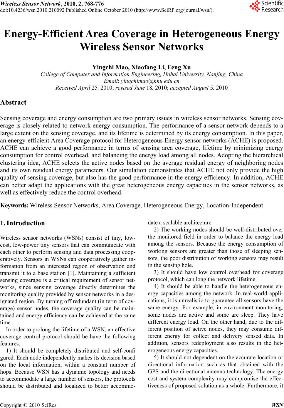Wireless Sensor Network, 2010, 2, 768-776
doi:10.4236/wsn.2010.210092 October 2010 (http://www.SciRP.org/journal/wsn/). Published Online
Energy-Efficient Area Coverage in Heterogeneous Energy
Wireless Sensor Networks
Yingchi Mao, Xiaofang Li, Feng Xu
College of Computer and Information Engineering, Hohai University, Nanjing, China
Received April 25, 2010; revised June 18, 2010; accepted August 5, 2010
Abstract
Sensing coverage and energy consumption are two primary issues in wireless sensor networks. Sensing cov-
erage is closely related to network energy consumption. The performance of a sensor network depends to a
large extent on the sensing coverage, and its lifetime is determined by its energy consumption. In this paper,
an energy-efficient Area Coverage protocol for Heterogeneous Energy sensor networks (ACHE) is proposed.
ACHE can achieve a good performance in terms of sensing area coverage, lifetime by minimizing energy
consumption for control overhead, and balancing the energy load among all nodes. Adopting the hierarchical
clustering idea, ACHE selects the active nodes based on the average residual energy of neighboring nodes
and its own residual energy parameters. Our simulation demonstrates that ACHE not only provide the high
quality of sensing coverage, but also has the good performance in the energy efficiency. In addition, ACHE
can better adapt the applications with the great heterogeneous energy capacities in the sensor networks, as
well as effectively reduce the control overhead.
Keywords: Wireless Sensor Networks, Area Coverage, Heterogeneous Energy, Location-Independent
1. Introduction
Wireless sensor networks (WSNs) consist of tiny, low-
cost, low-power tiny sensors that can communicate with
each other to perform sensing and data processing coop-
eratively. Sensors in WSNs can cooperatively gather in-
formation from an interested region of observation and
transmit it to a base station [1]. Maintaining a sufficient
sensing coverage is a critical requirement of sensor net-
works, since sensing coverage directly determines the
monitoring quality provided by sensor networks in a des-
ignated region. By turning off redundant (in term of cov-
erage) sensor nodes, the coverage quality can be main-
tained and energy efficiency can be achieved at the same
time.
In order to prolong the lifetime of a WSN, an effective
coverage control protocol should be have the following
features.
1) It should be completely distributed and self-confi
gured. Each node independently makes its decision based
on the local information, within a constant number of
hops. Because WSN has a dynamic topology and needs
to accommodate a large number of sensors, the protocols
should be distributed and localized to better accommo-
date a scalable architecture.
2) The working nodes should be well-distributed over
the monitored field in order to balance the energy load
among the sensors. Because the energy consumption of
working sensors are greater than those of sleeping sen-
sors, the poor distribution of working sensors may result
in the sensing hole.
3) It should have low control overhead for coverage
protocol, which can long the network lifetime.
4) It should be able to handle the heterogeneous en-
ergy capacities among the network. In real-world appli-
cations, it is unrealistic to guarantee all sensors have the
same energy. For example, in environment monitoring,
some nodes are active and some are sleep. They have
different energy load. On the other hand, due to the dif-
ferent position of active nodes, they may consume dif-
ferent energy for collect and delivery sensed data. In
addition, sensors redeployment also results in the het-
erogeneous energy capacities.
5) It should not dependent on the accurate location or
directional information such as that obtained with the
GPS and the directional antenna technology. The energy
cost and system complexity may compromise the effec-
tiveness of proposed solution as a whole. Furthermore, it

Y. C. MAO ET AL.769
is still a very difficult problem to estimate sensors’ loca-
tions, since GPS and other complicated hardware devices
consume too much energy and the costs are too high for
tiny sensors [2].
To meet the above requirements, an energy-efficient
location-independent area coverage protocol for hetero-
geneous energy sensor networks (ACHE) is proposed.
Different from DELIC [3], adopting the hierarchical clu-
stering idea, ACHE elects the working nodes based on
the average residual energy of neighboring nodes and its
own residual energy parameters. Simulation study dem-
onstrates that ACHE can better adapt the application with
the heterogeneous energy capacities and also effectively
reduce the control overhead.
The rest of the paper is organized as follows. In Sec-
tion 2, we will give a brief summary of the related work.
Section 3 describes the network model. Following that,
we present in Section 4 the proposed coverage protocol
ACHE. Section 5 will give the simulation and evaluation
results. Section 6 is the conclusion remarks.
2. Related Work
In [4] and [5], an approach is proposed to compute the
maximal cover set. The sensor nodes in each cover set
can perform independently the task of monitoring the
desired area; sensor nodes in all the cover sets take turns
at performing the monitoring task. The two algorithms
proposed are both centralized ones, so they are not suit-
able for the case in which there is a large quantity of
sensors.
In [6], Tian et al. propose a off-duty eligibility rule for
complete sensing coverage, relying on the geographical
information of sensor nodes and AOA (Arrival of Angle)
obtained through the directional antenna, can reckon the
coverage relation between one node and its neighbors
and then select working nodes. The off-duty eligibility
rule fails to consider the problem that excessive overlap
may be formed so that the number of working nodes se-
lected becomes very large to cause extra energy consum-
ption.
In [7], it is proved that to ensure that the full sensing
area coverage of a convex area also guarantee the con-
nectivity of the active nodes, the communication range
should be at least twice of the sensing range. Based on
the analytical results, Zhang et al. proposed a distributed,
localized density control algorithm named OGDC [7].
Wang et al. draw the same conclusion in [8], and pre-
sented a Coverage Configuration Protocol (CCP) that can
provide complete coverage. Based on OGDC, Wu et al.
proposed a coverage control protocol with adjustable
sensing range [9]. Every working node adjusts the ap-
propriate sensing range based on the relative position to
the neighboring nodes in order to decrease the excessive
overlap of sensing coverage.
The above coverage protocols have to rely on the lo-
cation information of sensor nodes in reckoning sensing
coverage. The following protocols do not require the
location information to solve the coverage problem.
Kumar et al. adopt the Randomized Independent Sche-
duling (RIS) mechanism [10]. At the beginning of each
round, each sensor independently decides whether to be-
come active with probability p or go to sleep with prob-
ability 1-p, p determines the network lifetime. Obviously,
RIS does not require location information and has no
communication overhead. But RIS is not robust against
unexpected failure before they run out of energy.
Ye et al. proposed a probing-based density control al-
gorithm named PEAS [11]. In PEAS, a sleeping node
wakes up periodically to probe its neighbors and transits
to working mode if there is no working node within its
probing range. Obviously, in PEAS, some nodes may die
too early and the energy consumption is unbalance, which
will severely affect the coverage quality.
Gao et al. propose a mathematical method, which does
not rely on location information, to describe the redun-
dancy [12]. According to this method, one sensor node
can utilize the number of neighbors within its sensing
range to calculate its own probability of becoming a re-
dundant node. However, for most sensor nodes, the sen-
sing hardware and the communicating hardware are two
fully independent parts, and the communicating range is
always not equal to the sensing range. Therefore, some
specialized parts are needed to judge the number of
neighbors within the sensing range.
Mao et al. proposed a location-independent coverage
protocol DELIC [3]. DELIC adopt the hierarchical clus-
tering mechanism for working sensor election by com-
paring its own residual energy to that of its neighboring
nodes. However, DELIC require several iteration to de-
termine final working sensors, which results the greater
control overhead.
Although the above protocols do not need the accurate
location information of sensors, they also have some limi-
tation. In addition, they could not discuss how to effec-
tively deal with the heterogeneous energy capacities for
coverage control.
3. Network Model
Assume N sensor nodes are randomly and uniformly dis-
tributed over the sensing field A. The sensor density is
high enough that any point of A can be monitored by
sensor nodes. We assume the following properties about
the wireless sensor network:
1) The nodes in the network are stationary and they
are left unattended after deployment.

Y. C. MAO ET AL. 770
2) For simplicity and convenience, the sensing mode is
Boolean mode.
3) All nodes should be roughly time synchronized on
the order of seconds.
4) All nodes have different initial energy and the bat-
tery could not be rechargeable.
5) Nodes are location-unaware, i.e. not equipped with
GPS-capable antennae.
6) Sensor’s radio transceiver is capable of changing its
transmission power in continuous steps to achieve dif-
ferent transmission ranges. Some sensors, such as the
MICAZ mote, provide multiple levels of transmission
power.
The first three properties are typical assumptions in
general wireless sensor networks. The forth property is
more suitable for the real-world application compared
with the same initial energy of all nodes. The fifth prop-
erty assumes the nodes are location-unaware, which can
decrease the hardware cost and energy consumption of
sensors. From the point of view of energy efficiency,
compared with the fix transmission power, the last prop-
erty can improve the energy efficiency to prolong the net-
work lifetime.
4. ACHE Protocol
In a WSN, the working sensors should receive and de-
livery the sensed data, which results in the higher energy
consumption than that of sleeping sensors. In order to
balance the energy load among the sensors in a WSN,
ACHE protocol involves round-operation. Each round
includes two phases: Decision phase and Sensing phase,
denoted by DT and ST respectively. In DT, based on the
hierarchical clustering idea, ACHE selects the working
nodes. First, every node exchange the information with
its neighbor nodes, then every node compete the working
node based on the average residual energy of neighbor
nodes and its own residual energy. After decision phase,
the working sensors can collect and delivery sensed data
to the base station, while other sensors enter into the
sleeping state.
4.1. Adjust Appropriate Transmission Range
In [13], we have given the theoretical analysis of the
sensing area coverage property of minimal dominating
set (MDS). Furthermore, we established the relationship
between point coverage and area coverage in random
geometric graphs.
Suppose sensor nodes follow Poisson point process of
density λ in the plane . According to (1), it can compute
the appropriate transmission range Rt.
2

RtRs r
2
((1) )
min( ,)
Rs
ln e
Rs Rs





 (1)
For 0


, any minimal dominating set of Gt (re-
call that Gt is a subgraph of G induced by transmission
range Rt) provides the same coverage as that of all sensor
nodes with probability at least1

.
On the other hand, Theorem 1 proves the set of
working nodes elected by ACHE must be a dominating
set in Subsection 4.3. Since MDS  CDS, we have
() ()
A
rea MDSArea DS

. By (1), every node can adjust
the appropriate transmission range Rt, according to the
local density λ, ACHE guarantee that the working nodes
can provide the high quality of sensing coverage.
With the execution of the sensor network, sensor
nodes are prone to fail, the value of λ is changing. For a
single node, it is very difficult to know the change of λ.
Therefore, each node determines a local node density
λlocal by counting the number of nodes in its k-hop neigh-
bors using the maximum transmission range. The
local node density λlocal can be approximated as the net-
work density λ and can be adapt to variations of node
density. The local node density λlocal can be computed as
follows:
maxRt
max 22
1
()
local
c
Rt k


 (2)
where |c| is the number of k-hop neighbors. The larger
the value of k is, the more accurate the approximation of
λlocal is. However, the increase of the number of messages
will results in the more energy consumption. ACHE es-
timates the local density λlocal by counting the number of
nodes in its 1-hop neighbor nodes usingma x
R
t.
Let . Clearly, . Comb-
ing the (1) and (2), we have
2
0(1 )Rs
e

 



00, 1
 
0
0
ln
min( ,)
min( ,)
||1
local
Rt RsRs
ln
RsRs c






 
(3)
Therefore, each sensor node can adjust the appropriate
the transmission range Rt by (3). The obtained sensing
coverage ratio has the probability at least1

.
4.2. Working Nodes Selection
Definition 1: Neighborhood. For any node Si, the
neighborhood node Sj of node Si is defined as
{( ,),}
jij
SdSSRtji

, where denotes the
distance between node S
i and node Sj, Rt denotes the
transmission range computed by (3).
(, )
ij
dS S
In order to effectively deal with the heterogeneous en-
ergy capacities in sensor networks, it is obvious that the

Y. C. MAO ET AL.771
higher energy the node has, the higher probability it be-
comes working nodes. Meanwhile, the lower average
energy of its neighborhood nodes, the higher probability
it becomes working nodes. Thus, ACHE elects the work-
ing nodes considering the parameters, the average resid-
ual energy of neighborhood nodes and the node own re-
sidual energy.
In ACHE, every node requires to maintain a neighbor-
hood table Neighbor_Table, recording the neighbors’ ID,
neighbors’ state, and neighbors’ residual energy. At the
beginning of each round, every node first broadcasts an
Energy_Msg message with the transmission range Rt to
its neighboring nodes. The Energy_Msg message in-
cludes ID of the sender node, state and its residual en-
ergy. Once receiving the Energy_Msg from its neighbor-
ring nodes, the node should update its own Neighbor_
Table. After updating its Neighbor_Table, every node
Si can compute the average residual energy of its neigh-
borring nodes, Si.Eavg. Let
1
.
.,(
m
jresidual
j
iavg
SE
SEi N
m



1) (4)
where m is the number of neighboring nodes of Si,
Sj.Eresidual (1 ≤ j ≤ m, j ≠ i) denotes the residual energy of
node Sj.
According to (4) and (5), we can obtain the time i
when the node Si broadcasts an Active_Msg message to
announce node Si would be a working node. An Ac-
tive_Msg message consists of ID of the sender node, and
its state ACTIVE.
t
.,(1 )
.
iavg
i
iresidual
SE
tkT iN
SE
 (5)
where k is a random uniformly distributed in [0.9, 1.0]; T
is the time length for selecting working nodes in each
round, that is T = DT; Si.Eresidual denotes the residual en-
ergy of node Si.
From (5), it can notice that ACHE protocol uses
as the main parameter for selecting
working nodes. That is to say, the time when the node
Si broadcasts an Active_Msg message is mainly deter-
mined by. Compared with DELIC
protocol, which is only based on its own residual energy
of node to compete the working node, ACHE can better
handle the heterogeneous energy capacities among the
sensor nodes.
./.
iavg ires idual
SE SE
./
iavg
SE
i
t
.
iresidual
SE
During the phase of selection working nodes, any node
Si checks whether it receives any Active_Msg from its
neighboring nodes before the timeiexpires. If node Si
gets the Active_Msg from neighbor node Sj before the
time i
texpires, node Si would lose the chance to become
the working node, and enter into the SLEEP state. That is
to say, node Si is in the sensing coverage of the neighbor
node Sj. If node Si does not receive any Active_Msg from
its neighboring nodes when the timeiexpires, which
means there is no neighbor node can cover the sensing
area of node Si, node Si broadcasts an Active_Msg to its
neighboring nodes, and becomes a working node and
changes its state to ACTIVE. However, if another
neighbor node Sk also broadcasts an Active_Msg message
between the time interval, there maybe
have several working nodes within each other’s trans-
mission range Rt.
t
t
t(,
ii
ttt )
t

is the time interval than all
neighboring nodes can receive Active_Msg message from
node Si in the worst case. Due to the short package and
limited broadcast range of Active_Msg message, t

is
quite small. Thus, the probability that several nodes
within the transmission range Rt are working nodes is
small. Theorem 3 would prove the result in Subsection
4.3.
From the above description for ACHE, it is clearly
found that there are only working nodes could broadcast
Active_Msg message, and every working node only
broadcast one Active_Msg message during the phase of
selecting working nodes, which can greatly reduce the
control overhead.
4.3. Protocol Analysis
ACHE is a completely distributed, self-configured sens-
ing coverage protocol. Node decisions are based solely
on local information. This section provides the theoreti-
cal analysis of ACHE for a better understanding.
Theorem 1: The set of working sensor nodes obtained
by ACHE forms a dominating set. That is to say, for any
sensor node v in the deployed sensor set N, node v is ei-
ther in the set of working sensor nodes or one of node v’s
neighbor nodes is in the set of working sensor nodes.
Proof: Randomly select a sensor node v in the de-
ployed sensor set N. If v is a working sensor node, Theo-
rem 1 holds. For the remaining case, we will show that
there exists a working neighboring sensor node of v.
Since v is not a working node, there exists at least one
working node u in the neighboring nodes of v.
Moreover, the time tu when node u broadcasts Ac-
tive_Msg message is earlier than that of node v. In an-
other words, before the time tv expires, v has received an
Active_Msg from u, and entered into the SLEEP state.
Otherwise, once the time tv expires, v has not received
any Active_Msg from its neighboring nodes, becomes a
working node, and broadcasts an Active_Msg to it
neighborhood.
Clearly, for any sensor node v in the deployed sensor
set N, node v is either in the set of working sensor nodes
or one of node v’s neighbor nodes is in the set of work-

Y. C. MAO ET AL. 772
ing sensor nodes.
Theorem 2: 0

 , the set of working sensor nodes
obtained by ACHE can provide the complete sensing
coverage with probability at least 1

.
Proof: In [13], we have proved that for0

 , any
minimal dominating set of Gt (Gt is a subgraph of G in-
duced by transmission range Rt based on (3)) provides
the same coverage as that of all sensor nodes with prob-
ability at least1

.
In the network model, it assumes that the sensor den-
sity is high enough that any point of A can be monitored
by sensor nodes. Since MDS  CDS, we have
() ()
A
rea MDSArea DS. According Theorem 1, the set
of working sensor nodes obtained by ACHE forms a
dominating set. Therefore,0

 , the set of working
sensor nodes obtained by ACHE can provide the com-
plete sensing coverage with probability at least1


.
Theorem 3: In each round, the probability that several
working nodes within one transmission range Rt is small,
i.e., working sensor nodes are well-distributed.
Proof: In ACHE protocol, every node must compete
for working node with its neighboring node. Assume that
after one node v broadcasts an Active_Msg message
within its transmission range Rt, it can guarantee that all
neighboring nodes can receive Active_Msg message
from node v in the intervalt

. Obviously, if no other
neighboring nodes of node v broadcast Active_Msg
message in the interval, node v becomes the only one
working node within its transmission range Rt. On the
other hand, if other neighboring nodes broadcast Ac-
tive_Msg in the interval , there maybe exist several
working nodes within one transmission range Rt. Con-
sider the probability that several working nodes within
one transmission range Rt, denoted as p.
t
t
According to (2), the time when any node broadcasts
an Active_Msg message is approximately random uni-
formly distributed in [0, T]. Therefore, the probability p
could satisfy the Equation (6).
0
1
1(1)
m
m
t
pC T


1

  (6)
where m-1 is the expected value of the number of sensor
nodes within the transmission range Rt.
Clearly,
2
Rt
m
A





N


s
. With typical values of other
parameters, the probability p is very small. For example,
Rt = 10 m, || A|| = (100 × 100) m2, N = 100, T = 10 s,
, the resulting p = 0.00214. 10tm
Therefore, the probability that several working nodes
within one transmission range Rt is small.
Theorem 4: ACHE has a worst case message ex-
change complexity of per node and of in
the network.
(1)O()ON
Proof: During the execution of ACHE, if node v re-
ceived the Active_Msg messages from its neighbouring
nodes before the time tv expires, node v enters into the
SLEEP state and does not send any message. Otherwise,
node v enters into the ACTIVE state and broadcasts an
Active_Msg message. Since the number of these Ac-
tive_Msg messages in the network is less than N, the
number of messages exchanged in the network is up-
per-bound by.
()ON
5. Simulation Study
5.1. Simulation Setup and Parameters
To evaluate the performance of the ACHE protocol, we
use GloMoSim [14] as the simulation platform in terms
of evaluating the number of working nodes, coverage
ratio, the network lifetime and control overhead. In the
simulation, 600-1200 sensors are randomly deployed in a
100 × 100 (m2) region, and each sensor has a sensing
range of 10 meters, the maximum transmission range of
20 meters. To demonstrate ACHE could better adapt
with the heterogeneous energy capacities in the sensor
networks than others, simulation setups three different
degree for heterogeneous energy among the sensor nodes.
The initial energy of sensor nodes in the network is ran-
domly uniformly distributed in (0.2 J, 2.0 J), (1.0 J, 2.0 J),
and (1.5 J, 2.0 J) respectively. To evaluate the perform-
ance of energy efficiency, we use the same network pa-
rameters and radio model as presented in [15].
In article [3], we have compared DELIC protocol with
other coverage protocols. DELIC protocol outperforms
the Sponsor area [6], OGDC, PEAS in term of coverage
ratio, energy efficiency and balancing energy load. Thus,
we only compare proposed ACHE with DELIC in our
simulation experiment.
5.2. Effectiveness of ACHE
Figure 1 and Figure 2 give the curves of the number of
working nodes and sensing coverage ratio in the different
deployed nodes density with the different degree of het-
erogeneous energy capacities. As shown in Figure 1 and
Figure 2, the number of working nodes obtained by
ACHE is smaller about 15% than that of DELIC in the
different nodes density. In the most situations, ACHE
can provide above 99% sensing coverage for the differ-
ent node density. But the quality of sensing coverage by
ACHE is little poorer than that of DELIC. For the most
application, the above 99% sensing coverage is accept-
able and reasonable. In addition, as the same with DELIC,
the number of working nodes by ACHE does not in-
crease with the number of deployed nodes. This is be-
cause the number of working nodes in ACHE is related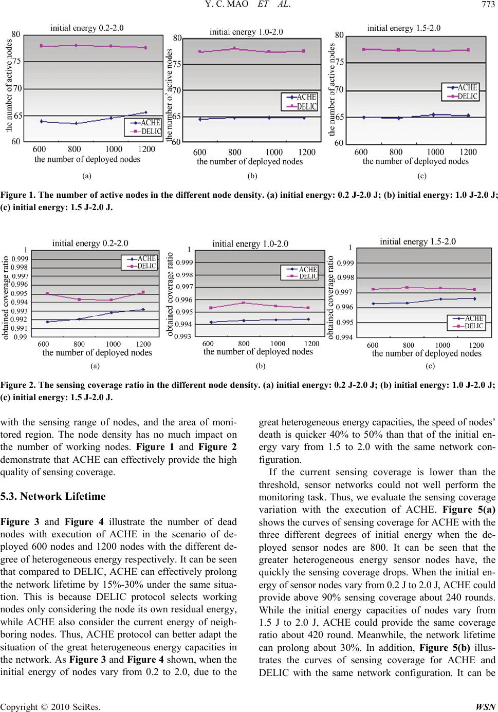

Y. C. MAO ET AL. 773
(a) (b) (c)
Figure 1. The number of active nodes in the different node density. (a) initial energy: 0.2 J-2.0 J; (b) initial energy: 1.0 J-2.0 J;
(c) initial energy: 1.5 J-2.0 J.
(a) (b) (c)
Figure 2. The sensing coverage ratio in the different node density. (a) initial energy: 0.2 J-2.0 J; (b) initial energy: 1.0 J-2.0 J;
(c) initial energy: 1.5 J-2.0 J.
with the sensing range of nodes, and the area of moni-
tored region. The node density has no much impact on
the number of working nodes. Figure 1 and Figure 2
demonstrate that ACHE can effectively provide the high
quality of sensing coverage.
5.3. Network Lifetime
Figure 3 and Figure 4 illustrate the number of dead
nodes with execution of ACHE in the scenario of de-
ployed 600 nodes and 1200 nodes with the different de-
gree of heterogeneous energy respectively. It can be seen
that compared to DELIC, ACHE can effectively prolong
the network lifetime by 15%-30% under the same situa-
tion. This is because DELIC protocol selects working
nodes only considering the node its own residual energy,
while ACHE also consider the current energy of neigh-
boring nodes. Thus, ACHE protocol can better adapt the
situation of the great heterogeneous energy capacities in
the network. As Figure 3 and Figure 4 shown, when the
initial energy of nodes vary from 0.2 to 2.0, due to the
great heterogeneous energy capacities, the speed of nodes’
death is quicker 40% to 50% than that of the initial en-
ergy vary from 1.5 to 2.0 with the same network con-
figuration.
If the current sensing coverage is lower than the
threshold, sensor networks could not well perform the
monitoring task. Thus, we evaluate the sensing coverage
variation with the execution of ACHE. Figure 5(a)
shows the curves of sensing coverage for ACHE with the
three different degrees of initial energy when the de-
ployed sensor nodes are 800. It can be seen that the
greater heterogeneous energy sensor nodes have, the
quickly the sensing coverage drops. When the initial en-
ergy of sensor nodes vary from 0.2 J to 2.0 J, ACHE could
provide above 90% sensing coverage about 240 rounds.
While the initial energy capacities of nodes vary from
1.5 J to 2.0 J, ACHE could provide the same coverage
ratio about 420 round. Meanwhile, the network lifetime
can prolong about 30%. In addition, Figure 5(b) illus-
trates the curves of sensing coverage for ACHE and
DELIC with the same network configuration. It can be
C
opyright © 2010 SciRes. WSN

Y. C. MAO ET AL. 774
(a) (b) (c)
Figure 3. Timing of the nodes’ death (600 nodes). (a) initial energy: 0.2 J-2.0 J; (b) initial energy: 1.0 J-2.0 J; (c) initial energy:
1.5 J-2.0 J.
(a) (b) (c)
Figure 4. Timing of the nodes’ death (1200 nodes). (a) initial energy: 0.2 J-2.0 J; (b) initial energy: 1.0 J-2.0 J; (c) initial en-
ergy: 1.5 J-2.0 J.
(a) (b)
Figure 5. The sensing coverage ratio vs. round. (a) initial energy: 0.2 J-2.0 J; (b) initial energy: 1.5 J-2.0 J.
seen that the curve of sensing coverage of ACHE de-
creases more slowly than that in DELIC. This is due to
the fact that ACHE can better adapt the heterogeneous
energy capacities among senor nodes than DELIC.
5.4. Control Overhead
For ACHE, first, each nodes needs to count the number
of 1-hop neighbors and adjust the appropriate transmis-
sion range. Thus, each node consumes energy to receive
and send control messages. Second, in the phase of work-
ing nodes selection, every node also broadcasts an En-
ergy_Msg message to its neighbor nodes to update the
Neighbor_Table. Moreover, every working node needs
to broadcast an Active_Msg message within its transmis-
sion range to announce its state. Therefore, the node
density could have an impact on the control overhead.
Figure 6 compares the control overhead in the differ-
ent node density with the different degrees of initial en-
ergy capacities between ACHE and DELIC. It is obvious
C
opyright © 2010 SciRes. WSN

Y. C. MAO ET AL. 775
(a) (b) (c)
Figure 6. Control overhead in the different node density. (a) initial energy: 0.2 J-2.0 J; (b) initial energy: 1.0 J-2.0 J; (c) initial
energy: 1.5 J-2.0 J.
that the higher node density, the more control overhead
in the same network configuration. In ACHE, the control
overhead with 600 nodes is about twice that with 1200
nodes. On the other hand, it can be seen that the hetero-
geneous energy capacities in the network do not have
great impact on the control overhead.
6. Conclusions
In this paper, an energy-aware location-independent co-
verage control protocol for heterogeneous wireless sen-
sor networks (ACHE) is proposed. ACHE can achieve a
good performance in terms of sensing coverage, lifetime
by minimizing energy consumption for control overhead,
and balancing the energy load among all nodes. Adopt-
ing the hierarchical clustering idea, ACHE elects the
working nodes based on the average residual energy of
neighboring nodes and its own residual energy parame-
ters. Our simulation study and analysis demonstrate that
ACHE not only provide the high quality of sensing cov-
erage, but also has the good performance in the energy
efficiency. In addition, ACHE can better adapt the ap-
plications with the great heterogeneous energy capacities
in the sensor networks, as well as effectively reduce the
control overhead.
7. Acknowledgements
This research is supported by the NSF of Hohai Univer-
sity under Grant No. 2008428911, and the Fundamental
Research Funds for the Central Universities 2009B20714.
8
. References
[1] I. F. Akyildiz, W Su, Y. Sankarasubramaniam and E.
Cayirci, “Wireless Sensor Networks: A Survey,” Com-
puter Networks, Vol. 38, No. 4, 2002, pp. 393-422.
[2] I. Stojmenovic, “Position Based Routing in Ad Hoc Net-
works,” IEEE Communications Magazine, Vol. 40, No. 7,
2002, pp. 128-134.
[3] Y. C. Mao, M. Liu, L. J. Chen and D. X. Chen, “A Dis-
tributed Energy-Efficient Location-Independent Coverage
Protocol in Wireless Sensor Networks,” Computer Resear-
ch and Development, Vol. 43, No. 2, 2006, pp. 187-195.
[4] S. Slijepcevic and M. Potkonjak, “Power Efficient Or-
ganization of Wireless Sensor Networks,” Proceedings of
IEEE Conference on Communications, Helsinki, 2001,
Vol. 2, pp. 472-476.
[5] M. Cardei, D. MarCallum, X. Cheng, M. Min, X. Jia, D.
Li, et al., “Wireless Sensor Networks with Energy Effi-
cient Organization,” Journal of Interconnection Networks,
Vol. 3, No. 3-4, 2002, pp. 213-229.
[6] D. Tian and N. D. Georganas, “A Coverage-Preserving
Node Scheduling Scheme for Large Wireless Sensor Net-
works,” Proceedings of 1st ACM International Workshop
on Wireless Sensor Networks and Applications, Atlanta,
2002, pp. 32-41.
[7] H. Zhang and J. C. Hou, “Maintaining Sensing Coverage
and Connectivity in Large Sensor Networks,” Interna-
tional Journal of Ad Hoc & Sensor Wireless Networks,
Vol. 1, No. 1-2, 2005, pp. 89-124.
[8] X. Wang, G. Xing, Y. Zhang, C. Lu, R. Pless and C. D.
Gill, “Integrated Coverage and Connectivity Configura-
tion in Wireless Sensor Networks,” Proceedings of the
1st International Conference on Embedded Networked
Sensor Systems, Los Angeles, 2003, pp. 28-39.
[9] T. T. Wu and K. F. Su, “Determining Active Sensor No-
des for Complete Coverage without Location Informa-
tion,” International Journal of Ad Hoc and Ubiquitous
Computing, Vol. 1, No. 1-2, 2005, pp. 38-46.
[10] S. Kumar, T. H. Lai and J. Balogh, “On K-Coverage in a
Mostly Sleeping Sensor Network,” Proceedings of the
10th Annual International Conference on Mobile Com-
puting and Networking, Philadelphia, 2004, pp. 144-158.
[11] F. Ye, G. Zhong, S. Lu and L. Zhang, “PEAS: A Robust
Energy Conserving Protocol for Long-Lived Sensor Net-
works,” Proceedings of the 23rd International Confer-
ence on Distributed Computing Systems, Providence, 2003,
pp. 28-37.
C
opyright © 2010 SciRes. WSN

Y. C. MAO ET AL. 776
[12] K. Wu, Y. Gao, F. Li and Y. Xiao, “Lightweight Deploy-
ment-Aware Scheduling for Wireless Sensor Networks,”
ACM/Kluwer Mobile Networks and Applications, Vol. 10,
No. 6, 2004, pp. 837-852.
[13] Y. C. Mao, G. F. Feng, L. J. Chen and D. X. Chen, “A
Location-Independent Connected Coverage Protocol for
Wireless Sensor Networks,” Journal of Software, Vol. 18,
No. 7, 2007, pp. 1672-1684.
[14] http://pcl.cs.ucla.edu/projects/glomosim/
[15] W. Heinzelman, “Application-Specific Protocol Archi-
tecture for Wireless Sensor Networks,” Ph.D. Thesis, Ma-
ssachusetts Institute of Technology, Boston, 2000.