Paper Menu >>
Journal Menu >>
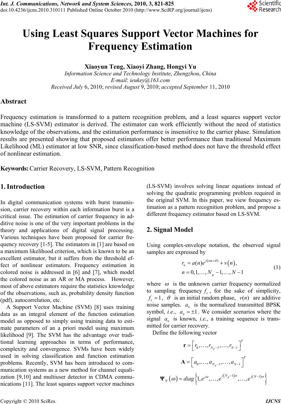 Int. J. Communications, Network and System Sciences, 2010, 3, 821-825 doi:10.4236/ijcns.2010.310111 Published Online October 2010 (http://www.SciRP.org/journal/ijcns) Copyright © 2010 SciRes. IJCNS Using Least Squares Support Vector Machines for Frequency Estimation Xiaoyun Teng, Xiaoyi Zhang, Hongyi Yu Information Science and Technolog y Institute, Zhengzhou, China E-mail: ieukey@163.com Received July 6, 2010; revised August 9, 2010; accepted September 11, 2010 Abstract Frequency estimation is transformed to a pattern recognition problem, and a least squares support vector machine (LS-SVM) estimator is derived. The estimator can work efficiently without the need of statistics knowledge of the observations, and the estimation performance is insensitive to the carrier phase. Simulation results are presented showing that proposed estimators offer better performance than traditional Maximum Likelihood (ML) estimator at low SNR, since classification-based method does not have the threshold effect of nonlinear estimation. Keywords: Carrier Recovery, LS-SVM, Pattern Recognition 1. Introduction In digital communication systems with burst transmis- sion, carrier recovery within each information burst is a critical issue. The estimation of carrier frequency in ad- ditive noise is one of the very important problems in the theory and applications of digital signal processing. Various techniques have been proposed for carrier fre- quency recovery [1-5]. The estimators in [1] are based on a maximum likelihood criterion, which is known to be an excellent estimator, but it suffers from the threshold ef- fect of nonlinear estimators. Frequency estimation in colored noise is addressed in [6] and [7], which model the colored noise as an AR or MA process. However, most of above estimators require the statistics knowledg e of the observations, such as, probability density function (pdf), autocorrelation, etc. A Support Vector Machine (SVM) [8] uses training data as an integral element of the function estimation model as opposed to simply using training data to esti- mate parameters of an a priori model using maximum likelihood [9]. The SVM has the advantage over tradi- tional learning approaches in terms of performance, complexity and convergence. SVMs have been widely used in solving classification and function estimation problems. Recently, SVM has been introduced to com- munication systems as a new method for channel equali- zation [9,10] and multiuser detector in CDMA commu- nications [11]. The least squares support vector machines (LS-SVM) involves solving linear equations instead of solving the quadratic programming problem required in the original SVM. In this paper, we view frequency es- timation as a pattern recognition problem, and propose a different frequency estimator based on LS-SVM. 2. Signal Model Using complex-envelope notation, the observed signal samples are expressed by () , 0,1, ,1, ,1 jn n p rane vn nNN (1) where is the unknown carrier frequency normalized to sampling frequency s f , for the sake of simplicity, 1 s f , is an initial random phase, ()vn are additive noise samples. n a is the normalized transmitted BPSK symbol, i.e., 1 n a . We consider scenarios where the signal n a is known, i.e., a training sequence is trans- mitted for carrier recovery. Define the following vector 011 ,, ,, p T NN rr r r 011 ,, ,, p T NN aa a A 11 1, ,,,, p jN jN j Ndiag eee Ψ  X. Y. TENG ET AL. Copyright © 2010 SciRes. IJCNS 822 0,1,,1 T vv vN v (2) The signal model can be arranged in matrix form as jN e rΨAv (3) 3. SVM Based Frequency Estimation 3.1. SVM Introduction SVM developed by Vapnik is a new type of learning machines which has a high generalization performance and sparse solution. It replaces empirical risk minimiza- tion by structural risk minimization (SRM). The goal of SVM is to find the hyperplane that maximizes the mini- mum distance between any point and the hyperplane. The idea of SVM can be expressed as follows. Consider (x ,),1,2,...., ii yi N be a linearly separa- ble training set, wherexd Rand {1,1}y , which can be separated by the hyperplane satisfying0 T wxb , where w is the weight vector and b is the bias. If this hyperplane maximizes the margin, then we need to solve the following optim izat ion probl em. 2 1 minimize 2 subject to 1 ii w ywx b (4) For the inputs data that is not separable, SVM uses soft margins that can be expressed as follows, by intro- ducing the non-negative slack variables , 1,..., iiN : 2 1 1 minimize 2 subject to ()1 lk i i T ii i C ywx b w (5) Data points are penalized if they are misclassified. The parameter C controls trad eoff between the complexity of the model and the classification errors. To construct nonlinear decision functions, SVM maps the training data nonlinearly into a higher-dimensional feature space via a kernel function, and constructs a separating hyperplane with maximum margin there. The kernel fun c tion is (, )()() T iji j K xxx x (6) The typical kernel functions include RBF , K xy 22 exp/ 2xy and polynomial , K xy 1d x y . We prefer LS-SVM over other models of SVM, for it offers a fast method for obtaining classifiers with good generalization performance in many applications. In LS-SVM, an equality constraint-based formulation is involved instead of the convex quadratic programming (QP) pro blem in (5). 22 1 1 minimize 2 subject to ()1 l i i T ii i C ywx b w (7) To solve this problem Lagrange multipliers (,1,..., ;0) ii il are used: 22 11 1()1 2 lN T P iiii i ii LC yb wwx (8) The KKT optimality conditions are give n by 1 1 00 00 00 010 l pii i i l pii i pii i pT ii i i i Lwyx w Ly b LC Lywx b (9) Optimal decision function (ODF) is then given by: 1 sign n ii i i f xyKxxb (10) 3.2. SVM-FEA To the best of our knowledge, SVM has not been im- plemented yet for parameter estimation in digital commu- nication systems. We introduce SVM as a new method for frequency estimation, by building the following frequency estimator 1 ˆargmin ; N n n (11) where the cost function () ;() () jn nrnesn (12) In such a scenario, the frequency estimation problem can be transferred to a pattern recognition problem. The optimal estimate of can be attained by minimizing the classification error. In a general way, the carrier phase existing in the received signal samples is unknown. Thus, the ideal ML detector is hard to handle the classification problem in (12). The powerful LS-SVM technique is applied in this paper. To fit the support vector machine model, the outpu t of the channel can be grouped into vectors x( )Re( ),Im( ) jn jn nrne rne (14) 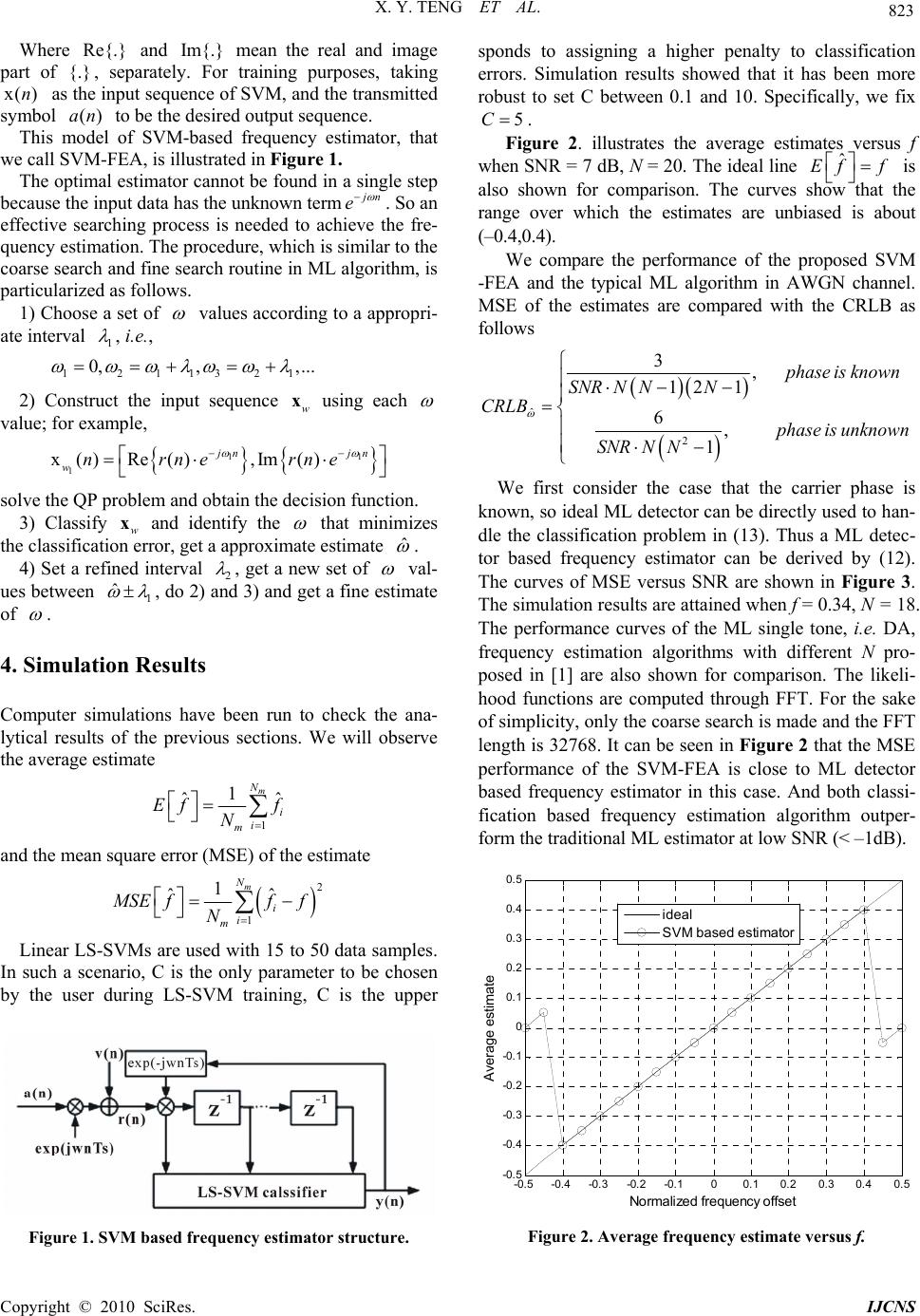 X. Y. TENG ET AL. Copyright © 2010 SciRes. IJCNS 823 Where Re{.} and Im{.} mean the real and image part of {.}, separately. For training purposes, taking x( )n as the input sequence of SVM, and the transmitted symbol ()an to be the desired output sequence. This model of SVM-based frequency estimator, that we call SVM-FEA, is illustrated in Figure 1. The optimal estimator cannot be found in a single step because the input data has the unknown term j n e . So an effective searching process is needed to achieve the fre- quency estimation. The procedure, which is similar to the coarse search and fine search routine in ML algorithm, is particularized as follows. 1) Choose a set of values according to a appropri- ate interval 1 , i.e., 1211321 0, ,,... 2) Construct the input sequence w x using each value; for example, 11 1 x()Re (),Im () jn jn wnrne rne solve the QP problem and obtain the decision function. 3) Classify w x and identify the that minimizes the classification error, get a approximate estimate ˆ . 4) Set a refined interval 2 , get a new set of val- ues between 1 ˆ , do 2) and 3) and get a fine estimate of . 4. Simulation Results Computer simulations have been run to check the ana- lytical results of the previous sections. We will observe the average estimate 1 1 ˆˆ m N i i m Ef f N and the mean square error (MSE) of the estimate 2 1 1 ˆˆ m N i i m M SE fff N Linear LS-SVMs are used with 15 to 50 data samples. In such a scenario, C is the only parameter to be chosen by the user during LS-SVM training, C is the upper Figure 1. SVM based frequency estimator structure. sponds to assigning a higher penalty to classification errors. Simulation results showed that it has been more robust to set C between 0.1 and 10. Specifically, we fix 5C . Figure 2. illustrates the average estimates versus f when SNR = 7 dB, N = 20. The ideal line ˆ Eff is also shown for comparison. The curves show that the range over which the estimates are unbiased is about (–0.4,0.4). We compare the performance of the proposed SVM -FEA and the typical ML algorithm in AWGN channel. MSE of the estimates are compared with the CRLB as follows ˆ 2 3, 12 1 6, 1 phase is known SNR NNN CRLB phase is unknown SNR NN We first consider the case that the carrier phase is known, so ideal ML detector can be directly used to han- dle the classification problem in (13). Thus a ML detec- tor based frequency estimator can be derived by (12). The curves of MSE versus SNR are shown in Figure 3. The simulation results are attained when f = 0.34, N = 18. The performance curves of the ML single tone, i.e. DA, frequency estimation algorithms with different N pro- posed in [1] are also shown for comparison. The likeli- hood functions are computed through FFT. For the sake of simplicity, only the coarse search is made and the FFT length is 32768. It can be seen in Figure 2 that the MSE performance of the SVM-FEA is close to ML detector based frequency estimator in this case. And both classi- fication based frequency estimation algorithm outper- form the traditional ML estimator at low SNR (< –1dB). -0.5 -0.4 -0.3-0.2 -0.1 00.1 0.20.3 0.4 0.5 -0.5 -0.4 -0.3 -0.2 -0.1 0 0.1 0.2 0.3 0.4 0.5 N or m alized fr equen c y off set Average est imat e ideal SVM base d es t im at o r Figure 2. Average frequency estimate versus f. 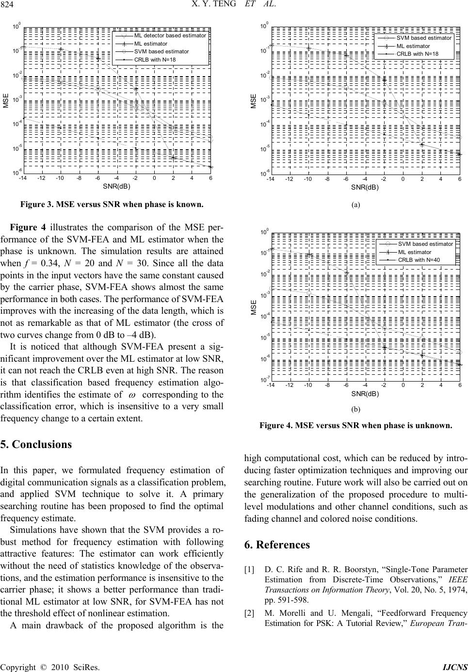 X. Y. TENG ET AL. Copyright © 2010 SciRes. IJCNS 824 -14 -12 -10-8-6-4-20 24 6 10 -6 10 -5 10 -4 10 -3 10 -2 10 -1 10 0 SNR( dB) MS E ML detector bas ed estim ator ML est imator SVM bas ed esti mator CRLB with N=1 8 Figure 3. MSE versus SNR when phase is known. Figure 4 illustrates the comparison of the MSE per- formance of the SVM-FEA and ML estimator when the phase is unknown. The simulation results are attained when f = 0.34, N = 20 and N = 30. Since all the data points in the input vectors have the same constant caused by the carrier phase, SVM-FEA shows almost the same performance in both cases. The performance of SVM-FEA improves with the increasing of the data length, which is not as remarkable as that of ML estimator (the cross of two curves change from 0 dB to –4 dB). It is noticed that although SVM-FEA present a sig- nificant improvement over the ML estimator at low SNR, it can not reach the CRLB even at high SNR. The reason is that classification based frequency estimation algo- rithm identifies the estimate of corresponding to the classification error, which is insensitive to a very small frequency change to a certain extent. 5. Conclusions In this paper, we formulated frequency estimation of digital communication signals as a classification problem, and applied SVM technique to solve it. A primary searching routine has been proposed to find the optimal frequency estimate. Simulations have shown that the SVM provides a ro- bust method for frequency estimation with following attractive features: The estimator can work efficiently without the need of statistics knowledge of the observa- tions, and the estimation performance is insensitive to the carrier phase; it shows a better performance than tradi- tional ML estimator at low SNR, for SVM-FEA has not the threshold effect of nonlinear estimation. A main drawback of the proposed algorithm is the -14 -12-10-8 -6-4 -20 2 4 6 10 -6 10 -5 10 -4 10 -3 10 -2 10 -1 10 0 SNR(dB) MS E S VM b ased esti mator ML estimator CRLB with N=18 (a) -14 -12-10-8 -6-4 -202 46 10 -7 10 -6 10 -5 10 -4 10 -3 10 -2 10 -1 10 0 SNR(dB) MS E S V M based estim ator ML estimator CRLB wi th N=4 0 (b) Figure 4. MSE versus SNR when phase is unknown. high computational cost, which can be reduced by intro- ducing faster optimization techniques and improving our searching routine. Future work will also be carried out on the generalization of the proposed procedure to multi- level modulations and other channel conditions, such as fading channel and colored noise conditions. 6. References [1] D. C. Rife and R. R. Boorstyn, “Single-Tone Parameter Estimation from Discrete-Time Observations,” IEEE Transactions on Information Theory, Vol. 20, No. 5, 1974, pp. 591-598. [2] M. Morelli and U. Mengali, “Feedforward Frequency Estimation for PSK: A Tutorial Review,” European Tran-  X. Y. TENG ET AL. Copyright © 2010 SciRes. IJCNS 825 sactions on Telecommunications, Vol. 9, No. 2, 1998, pp. 103-116. [3] W. Y. Kuo and M. P. Fitz, “Frequency Offset Compensation of Pilot Symbol Assisted Modulation in Frequency Flat Fading,” IEEE Transactions on Communications, Vol. 45, No. 11, 1997, pp. 1412-1416. [4] U. Mengali and M. Morelli, “Data-Aided Frequency Estimation for Burst Digital Transmission,” I E E E Transactions on Communications, Vol. 45, No. 1, 1997, pp. 23-25. [5] Y. Wang, E. Serpedin and P. Ciblat, “Optimal Blind Carrier Recovery for MPSK Burst Transmissions,” IEEE Transactions on Communications, Vol. 51, No. 9, 2003, p p. 1571-1581. [6] D. N. Swingler, “Approximate Bounds on Frequency Estimaties for Short Cissoids in Colored Noise,” IEEE Transactions on Signal Processing, Vol. 46, No. 5, 1998, pp. 1456-1458. [7] J. Viterbi and A. M. Viterbi, “Nonlinear Estimation of Psk-Modulated Carrier Phase with Application to Burst Digital Transmissions,” IEEE Transactions on Information Theory, Vol. 29, No. 4, 1983, pp. 543-551. [8] V. N. Vapnik, “Statistical learning theory,” John Wiley & Sons, Inc., New York, 1998. [9] D. J. Sebald, “Support Vector Machine Techniques for Nonlinear Equalization,” IEEE Transactions on Signal Processing, Vol. 48, No. 11, 2000, pp. 3217-3226. [10] S. Chen, S. Gunn and C. Harris, “Decision Feedbach Equalizer Design Using Support Vector Machines,” Vision, Image and Signal Processing, Vol. 147, No. 3, 2000, pp. 213-219. [11] F. Perez-Cruz, A. Navia-Vazquez, P. Alarcon-Dianna and A. Artes-Rodriguez, “SVC-Based Equalizer for Burst TDMA Transmission,” Signal Processing, Vol. 81, No. 6, 2001, pp. 1681-1693. [12] J. G. Proakis, “Digital Communications,” 4th Edition, McGraw-Hill, New York, 2001. |