J. Biomedical Science and Engineering, 2013, 6, 236-248 JBiSE
http://dx.doi.org/10.4236/jbise.2013.62A029 Published Online February 2013 (http://www.scirp.org/journal/jbise/)
A novel over-sampling method and its application to
miRNA prediction
Xuan Tho Dang1*, Osamu Hirose2, Thammakorn Saethang1, Vu Anh Tran1, Lan Anh T. Nguyen1,
Tu Kien T. Le1, Mamoru Kubo2, Yoichi Yamada2, Kenji Satou2
1Graduate School of Natural Science and Technology, Kanazawa University, Kanazawa, Japan
2Institute of Science and Engineering, Kanazawa University, Kanazawa, Japan
Received 15 December 2012; revised 14 January 2013; accepted 20 January 2013
ABSTRACT
MicroRNAs (miRNAs) are short (~22 nt) non-coding
RNAs that play an indispensable role in gene regula-
tion of many biological processes. Most of current
computational, comparative, and non-comparative
methods commonly classify human precursor micro-
RNA (pre-miRNA) hairpins from both genome pseudo
hairpins and other non-coding RNAs (ncRNAs). Al-
though there were a few approaches achieving prom-
ising results in applying class imbalance learning
methods, this issue has still not so lved completely and
successfully yet by the existing methods because of
imbalanced class distribution in the datasets. For
example, SMOTE is a famous and general over-sam-
pling method addressing this problem, however in
some cases it cannot improve or sometimes reduces
classification performance. Therefore, we developed a
novel over-sampling method named incre-mental-
SMOTE to distinguish human pre-miRNA hairpins
from both genome pseudo hairpins and other ncRNAs.
Experimental results on pre-miRNA datasets from
Batuwita et al. showed that our method achieved bet-
ter Sensitivity and G-mean than the control (no over-
sampling), SMOTE, and several successsors of modi-
fied SMOTE including safe-level-SMOTE and bor-
der-line-SMOTE. In addition, we also applied the
novel method to five imbalanced benchmark datasets
from UCI Machine Learning Repository and ach-
ieved improvements in Sensitivity and G-mea n. These
results suggest that our method outperforms SMOTE
and several successors of it in various biomedical
classification problems including miRNA classifica-
tion.
Keywords: Imbalanced Dataset; Over-Sampling;
SMOTE; miRNA Classification
1. INTRODUCTION
MicroRNAs (miRNAs) are short (~22nt) non-coding
RNAs (ncRNAs) that play an indispensable role in gene
regulation of many biological processes. The tiny miRNAs
can target numerous mRNAs to induce mRNA degrada-
tion or translational repression or both, they could regulate
20% - 30% of human genes [1]. The miRNAs are tran-
scribed as long primary miRNAs (pri-miRNAs) which are
processed into 60 - 70 nt precursor miRNAs (pre-
miRNAs) by Drosha-DGCR8. The pre-miRNA is trans-
ferred from Nucleus to Cytoplasm by Exp5-RanGTP and
then split by Dicer-TRBP into miRNA duplex (~22 nt) [1].
The first miRNAs were characterized in early 1990s [2]
but research on miRNAs has not revealed multiple roles
in gene regulation (transcript degradation, translational
suppression or transcriptional and translational activation)
yet. Until the early 2000s, miRNAs were recognized as
essential components in most biological processes [3-6].
Subsequently, miRNAs have become a hot topic and a
large number of miRNAs, particularly 21,264 different
miRNAs have been identified in various species so far
according to the release 19 of miRBase [7]. However, the
identification of miRNAs from a genome by existing
experiment techniques is so difficult, expensive, and re-
quires a large amount of time. Therefore, computational
methods with two main approaches based on compara-
tive and non-comparative methods play important role to
detect new miRNAs. The rationale idea of the first ap-
proach—comparative methods is that miRNA genes are
conserved in closely related genomes in hairpin second-
dary structures. Several comparative methods are pre-
sented such as RNAmicro [8], MiRscan [9], miRseeker
[10], MIRcheck [11], and MiRFinder [12]. These con-
servation-dependent comparative methods are successful
to predict hundreds of miRNAs with high sensitivity in
closely related species. However, they are unable to
identify novel miRNAs without close homologies due to
lack of current data or unreliability of alignment algo-
rithms [13], especially due to possibly rapid evolution of
*Corresponding author.

X. T. Dang et al. / J. Biomedical Science and Engineering 6 (2013) 236-248 237
miRNAs. Particularly, the report from Berezikov et al.
[14] has emphasized that non-conserved miRNAs in hu-
man genome missed by comparative methods are rela-
tively large and even have not still been recognized yet.
Meanwhile, the second approach—non-comparative
methods are promising for recognizing additional
miRNAs which are non-conserved miRNAs. The main
idea of these methods is based on hairpin secondary
structures of pre-miRNAs. Sewer et al. [15] used clus-
tering approach to predict novel miRNAs in the same
cluster with known miRNAs. Xue et al. [16] proposed
the classification of real and pseudo pre-miRNA hairpins
based on 32 features of structure-sequence triplet. Clote
et al. [17] and Hertel et al. [8] also identified that hairpin
secondary structures are popular in many types of
ncRNAs and a huge number of pseudo hairpins and hair-
pin structures can be found among secondary structures
of other ncRNAs. In addition, machine learning ap-
proaches including random forest prediction model [18,
19]; hybrid of genetic algorithm and support vector ma-
chine (GA-SVM) [20]; feature selection strategies based
on SVM and boosting method [21]; hidden Markov
model (HMM) [22] have also been used.
Therefore, both genome pseudo hairpins, other
ncRNAs and machine learning approaches should be
applied. In addition, miRNA prediction problem should
be also considered as imbalance class distribution. Batu-
wita et al. [23] proposed an effective classifier system,
namely microPred which used a complete pseudo hairpin
dataset and ncRNAs. In their research, they focused on
handling with class imbalance problem in datasets where
samples from the majority class (9248 = 8494 pseudo
hairpins + 754 other ncRNAs) significantly outnumber
the minority class (691 pre-miRNAs). Xiao et al. [24]
presented several network parameters based on two-di-
mensional network of pre-miRNA secondary structure
such as bracketed, tree, dual graph, etc. Their dataset
contained 3928 positive samples (animal pre-miRNAs)
and 8897 negative samples (8487 pseudo hairpins and
410 ncRNAs). Therefore, this dataset is suffered from
imbalance problem, that is, the negative dataset outnum-
bers the positive dataset. The main problem of class im-
balance distribution is that normal learners are often bi-
ased to the majority class, leading to good classification
for the majority class samples while misclassification for
many minority class ones. In order to solve these class
imbalance learning problems, some solutions have been
developed, including two main types: the external meth-
ods at data processing level and the internal methods at
algorithm level. One of remarkable solutions is SMOTE
which is a famous and general over-sampling method
addressing this problem. For example, experimental re-
sults of Batuwita et al. [23] suggested that the best clas-
sifier has been developed by applying the SMOTE
method. However, there are still some drawbacks of
SMOTE, particularly in some cases it cannot improve or
sometimes reduces classification performance. Therefore,
in our research we developed a novel over-sampling
method to achieve better classification performance than
both of the control method (no over-sampling) and
SMOTE in the classification of pre-miRNAs for human
miRNA gene prediction. Moreover, in order to demon-
strate the applicability of our methods, we also compare
our methods with several successors of modified
SMOTE including safe-level-SMOTE [25] and border-
line-SMOTE [26].
The structure of this paper is organized as follows:
Section 2 gives a brief introduction to SMOTE and some
related works, then shows its drawback; Section 3 intro-
duces three variations of our novel method, incremental-
SMOTE, which is improved from SMOTE; Section 4
analyses the experiments and compares our novel me-
thod with the control, SMOTE, safe-level-SMOTE, and
borderline-SMOTE methods. Finally, conclusions are
described in Section 5.
2. METHOD
2.1. SMOTE
Chawla et al. developed a minority over-sampling tech-
nique called SMOTE [27] in which the minority class
samples are over-sampled by creating synthetic samples
rather than by over-sampling with replacement. SMOTE
provided a new approach to over-sampling and intro-
duced a bias towards the minority class. The results in
[27] showed that this approach could improve the per-
formance of classifiers for the minority class.
In a less application-specific manner, synthetic sam-
ples are generated by operating in “feature space” rather
than “data space”. The minority class is over-sampled by
synthesizing new samples along the line joining the mi-
nority samples and their nearest neighbors. Depending
on the requirement of over-sampling amount, nearest
neighbors are selected by chance. Synthetic samples are
generated in the following way: firstly, compute the dif-
ference of feature vector between each minority class
sample and its randomly selected nearest neighbor. Then,
multiply this difference by a random number between 0
and 1, and finally add it to the feature vector of the mi-
nority sample. In this way, the synthetic minority sample
is generated along the line segment between two specific
features.
This approach is effective in forcing the decision re-
gion of the minority class to become more general as
shown in Figure 1. Figure 1(a) presents a typical case of
imbalanced data where samples from the majority class
greatly outnumber the minority class. As a result, the
majority class samples are well-classified whereas many

X. T. Dang et al. / J. Biomedical Science and Engineering 6 (2013) 236-248 238
thetic samples are generated between two sets of minor-
ity class samples named Source (S) and Destination (D).
Figure 2(b) describes step by step the generation of syn-
thetic samples by using SMOTE method: at the first step,
a set of synthetic samples (X1) is generated, and at the
next step, another new set (X2) is generated; the process
is repeated and the sets of generated synthetic samples
can be different in each step.
samples from the minority class are easy to be misclassi-
fied. Therefore, imbalanced dataset problem requires a
new and more adaptive method such as SMOTE. Figure
1(b) describes synthetic samples generated by SMOTE
to achieve more balanced distribution so that the classi-
fier recognizes all samples correctly.
A variation of SMOTE, namely borderline-SMOTE is
proposed by Han et al. [26] as the improvement of
SMOTE. The authors analyzed most of the classification
algorithms and attempt to learn the borderline of each
class as exactly as possible in the training process. Those
samples far from the borderline may make a little con-
tribution to classification. Therefore, their method was
based on the same over-sampling technique to SMOTE,
but the difference is it only over-sampled the borderline
samples of minority class instead of over-sampling all
samples of the class as in SMOTE.
In Figure 2(b), we could realize the drawbacks of
SMOTE method: S and D do not change in the process
of generating synthetic samples; and synthetic minority
class samples will not be paid any attention after they are
generated. Therefore, in order to address these drawbacks
and improve classification accuracy of the SMOTE me-
thod, we focus on how to utilize generated synthetic sam-
ples as members of Source and Destination sets for further
generation. This idea will be presented in next section, a
novel method namely incremental- SMOTE.
Another modification of SMOTE, safe-level-SMOTE
is also presented by Bunkhumpornpat et al. [25]. Instead
of randomly synthesizing the minority samples along the
line joining a minority sample and its selected nearest
neighbours, this method ignored nearby majority samples.
The safe-level-SMOTE method carefully generated syn-
thetic samples along the same line with different weight
level, called safe level. The safe level was computed by
using nearest neighbour minority samples.
Moreover, although X is generated by S and D, S is
the decisive factor in generating X. In contrast, D is only
a randomly selected nearest neighbor to be used in com-
bination with S in this generation. Therefore, the change
of S will lead to the change of X as shown below in in-
cremental-SMOTE2 and incremental-SMOTE3.
Based on the analysis, we present three new methods,
incremental-SMOTE1, incremental-SMOTE2, and incre-
mental-SMOTE3.
Although SMOTE and several successors of modified
SMOTE including borderline-SMOTE and safe-level-
SMOTE are famous and general over-sampling methods
addressing the imbalanced class distribution problems, in
some cases they cannot improve or sometimes reduce
classification accuracy.
2.3. Incremental-SMOTE1
The idea of incremental-SMOTE1 is simple: the Des-
tination set is expanded incrementally while keeping the
Source set to be unchanged in all steps. Figure 3 illus-
trates more details about this idea. In step 1, using
SMOTE, a set of synthetic samples X1 is generated from
two sets—Source (S) and Destination (D) sets as men-
tioned above. In step 2, the Destination set is expanded
by merging X1 into it. Similarly in step 3, the Destina-
tion set is expanded again by merging X2 into it. The
process is repeated in further steps.
2.2. Drawback of SMOTE
As discussed above, one particular synthetic sample is
generated by using SMOTE as shown in Figure 2(a).
Blue sample x is a synthetic sample generated along the
line joining a minority class sample s and its randomly
selected nearest neighbor d. Generally, the set of syn-
(a) (b)
Figure 1. Advantages of SMOTE. Black, red, and blue dots indicate majority class samples,
minority class samples, and synthetic minority class samples, respectively. The discrimina-
tion hyperplane is the brown line. (a) The original dataset with an erroneous classifier biased
by the imbalanced dataset; (b) Synthesize some new minority class samples by applying
SMOTE with a perfect classifier.

X. T. Dang et al. / J. Biomedical Science and Engineering 6 (2013) 236-248 239
(a) (b)
Figure 2. Synthetic samples generated normally by SMOTE. Both red and blue dots indicate
minority class samples. The latter indicate synthetic minority class samples generated by
using SMOTE. (a) Particularly, one synthetic minority class sample is generated along the
line of two minority class samples by using SMOTE; (b) Generally, a set of synthetic sam-
ples is generated from two sets named Source (S) and Destination (D).
Figure 3. The idea of incremental-SMOTE1.
Pseudo-code of incremental-SMOTE1 is as follows:
Algorithm incremental-SMOTE1 (T, N).
Input: The number of minority class samples T; Am-
ount of incremental-SMOTE1 N (%);
Output: (N × T/100) synthetic minority class samples
0) Initialize and assign two new sets with the same
size as the number of minority class samples.
Source = T; Destination = T;
1) Generate the new set X of T synthetic samples by
using SMOTE.
X = new synthetic samples generated at this step;
2) Merge X into the Destination set.
Destination = Destination + X;
3) Repeat from Step 1 N/100 times.
2.4. Incremental-SMOTE2
Incremental-SMOTE2 is based on a reversal idea: the
Destination set now is kept to be the same in every step,
and the Source set is expanded incrementally. It is shown
clearly in Figure 4.
Pseudo-code of incremental-SMOTE2 is as follows:
Algorithm incremental-SMOTE2 (T, N).
Input: The number of minority class samples T;
Amount of incremental-SMOTE2 N (%);
Output: (N × T/100) synthetic minority class samples
0. Initialize and assign two new sets with the same size
as the number of minority class samples.
Source = T; Destination = T;
1) Generate the new set X of T synthetic samples by
using SMOTE.
X = new synthetic samples generated at this step;
2) Merge X into the Source set.
Source = Source + X;
3) Repeat from Step 1 until (N × T/100) synthetic mi-
nority class samples are generated.
2.5. Incremental-SMOTE3
The idea of incremental-SMOTE3 is the combination of
incremental-SMOTE1 and incremental-SMOTE2: both
Source and Destination sets are expanded. Figure 5
shows more details for this idea.
Pseudo-code of incremental-SMOTE3 is as follows:
Algorithm incremental-SMOTE3 (T, N).
Input: The number of minority class samples T;
Amount of SMOTE N (%);
Output: (N * T/100) synthetic minority class samples
0) Initialize and assign two new sets with the same
size as the number of minority class samples.

X. T. Dang et al. / J. Biomedical Science and Engineering 6 (2013) 236-248 240
Figure 4. The idea of incremental-SMOTE2.
Figure 5. Thes idea of incremental-SMOTE3.
Source = T; Destination = T;
1) Generate the new set X of T synthetic samples by
using SMOTE.
X = new synthetic samples generated at this step;
2) Merge X into the Source and Destination sets.
Source = Source + X;
Destination = Destination + X;
3) Repeat from Step 1 until (N × T/100) synthetic mi-
nority class samples are generated.
2.6. Classifier
For binary class classification, Support Vector Machine
(SVM) is widely used to build a classifier discriminating
the classes [28]. SVM is based on simple ideas origi-
nated in statistical learning theory [29] which has high
generalization capability, optimizes global classification
solution and could be successfully applied in bioinfor-
matics. In addition, in order to more generally evaluate
the performance of our method, two different classifica-
tion methods other than SVM were used, namely k-
Nearest Neighbour (k-NN) and Random Forest (RF).
Implementation of SVM, k-NN, and RF in kernlab
[30], class [31], and random Forest [32]package avail-
able at the Comprehensive R Archive Network (CRAN)
was used, respectively. In our research, we used Radial
Basis kernel (Gaussian kernel) of kernlab for SVM.
Kernlab is an extensible package for kernel-based ma-
chine learning methods in R and includes various kernels
such as Linear kernel, Radial Basis kernel (Gaussian
kernel), Polynomial kernel, etc. Moreover, all hyper-
parameters for k-NN and RF, as well as other hyper-pa-
rameters for SVM such as cost, class weights, etc. were
also set to be default values.
2.7. Evaluation Measures
A confusion matrix of binary class classification is
shown in Ta bl e 1. In the field of binary classification in
imbalanced data, most of the studies consider the class
label of the minority class as positive. Thus, the class
labels positive and negative are given to the samples in
minority and majority classes, respectively. In Tab le 1,
the first column presents the actual class label of the
samples, and the first row is their predicted outcome
class label. TP and TN denote the number of positive and
negative samples that are classified correctly, while FN
and FP denote the number of misclassified positive and
negative samples, respectively.
If the dataset is extremely imbalanced, for example,
with an imbalance ratio of 99 to 1, even when the classi-
fier classifies all the samples as negative, the accuracy of
classification is still high up to 99%. As a result, accu-
racy is not used to evaluate the performance of classifier
for imbalance datasets, and more reasonable evaluation
metrics should be presented [33,34].
In medical science, bioinformatics, and machine lear-
ning communities [23,24,33,34], the sensitivity (SE) and
the specificity (SP) are two metrics used to evaluate the
performance of classifiers. Sensitivity measures the pro-
portion of actual positives which are correctly identified
as such, while specificity can be defined as the propor-
tion of negatives which are correctly identified. Kubat et
al. [35] proposed the Geometric mean metric defined as
follows.
G-mean =SE SP
There are many researches applying this metric for
evaluating classifiers as commonly used in imbalanced
Table 1. A confusion matrix for binary class classification.
Predicted Positive Predicted Negative
Observed Positive TP FN
Observed NegativeFP TN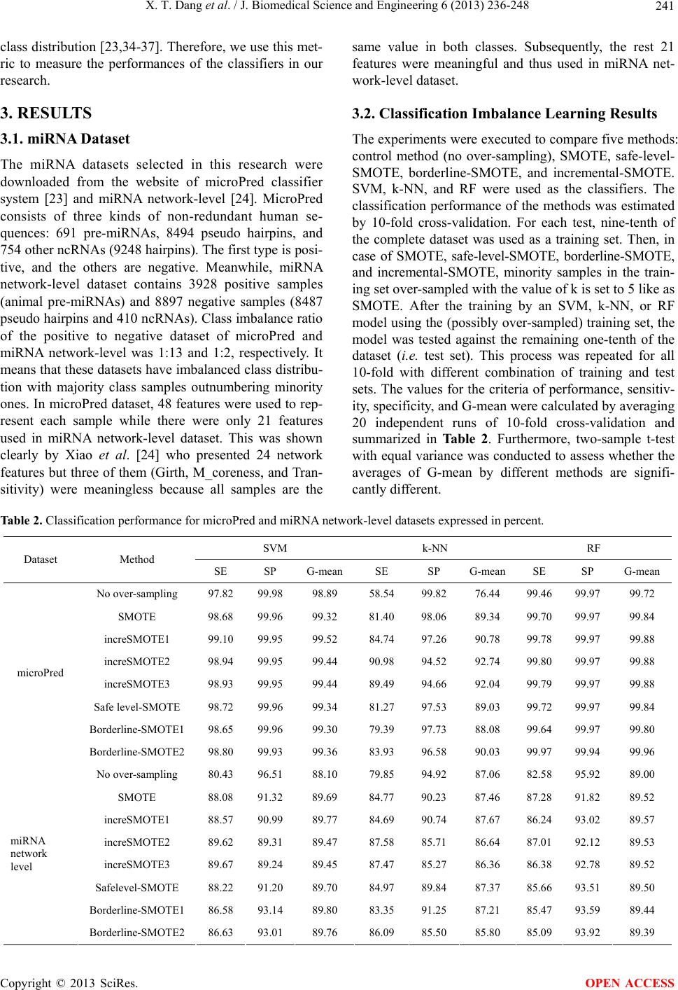

X. T. Dang et al. / J. Biomedical Science and Engineering 6 (2013) 236-248 241
class distribution [23,34-37]. Therefore, we use this met-
ric to measure the performances of the classifiers in our
research.
3. RESULTS
3.1. miRNA Dataset
The miRNA datasets selected in this research were
downloaded from the website of microPred classifier
system [23] and miRNA network-level [24]. MicroPred
consists of three kinds of non-redundant human se-
quences: 691 pre-miRNAs, 8494 pseudo hairpins, and
754 other ncRNAs (9248 hairpins). The first type is posi-
tive, and the others are negative. Meanwhile, miRNA
network-level dataset contains 3928 positive samples
(animal pre-miRNAs) and 8897 negative samples (8487
pseudo hairpins and 410 ncRNAs). Class imbalance ratio
of the positive to negative dataset of microPred and
miRNA network-level was 1:13 and 1:2, respectively. It
means that these datasets have imbalanced class distribu-
tion with majority class samples outnumbering minority
ones. In microPred dataset, 48 features were used to rep-
resent each sample while there were only 21 features
used in miRNA network-level dataset. This was shown
clearly by Xiao et al. [24] who presented 24 network
features but three of them (Girth, M_coreness, and Tran-
sitivity) were meaningless because all samples are the
same value in both classes. Subsequently, the rest 21
features were meaningful and thus used in miRNA net-
work-level dataset.
3.2. Classification Imbalance Learning Results
The experiments were executed to compare five methods:
control method (no over-sampling), SMOTE, safe-level-
SMOTE, borderline-SMOTE, and incremental-SMOTE.
SVM, k-NN, and RF were used as the classifiers. The
classification performance of the methods was estimated
by 10-fold cross-validation. For each test, nine-tenth of
the complete dataset was used as a training set. Then, in
case of SMOTE, safe-level-SMOTE, borderline-SMOTE,
and incremental-SMOTE, minority samples in the train-
ing set over-sampled with the value of k is set to 5 like as
SMOTE. After the training by an SVM, k-NN, or RF
model using the (possibly over-sampled) training set, the
model was tested against the remaining one-tenth of the
dataset (i.e. test set). This process was repeated for all
10-fold with different combination of training and test
sets. The values for the criteria of performance, sensitiv-
ity, specificity, and G-mean were calculated by averaging
20 independent runs of 10-fold cross-validation and
summarized in Table 2. Furthermore, two-sample t-test
with equal variance was conducted to assess whether the
averages of G-mean by different methods are signifi-
cantly different.
Table 2. Classification performance for microPred and miRNA network-level datasets expressed in percent.
SVM k-NN RF
Dataset Method
SE SP G-mean SE SP G-meanSE SP G-mean
No over-sampling 97.82 99.98 98.89 58.54 99.82 76.44 99.46 99.97 99.72
SMOTE 98.68 99.96 99.32 81.40 98.06 89.34 99.70 99.97 99.84
increSMOTE1 99.10 99.95 99.52 84.74 97.26 90.78 99.78 99.97 99.88
increSMOTE2 98.94 99.95 99.44 90.98 94.52 92.74 99.80 99.97 99.88
increSMOTE3 98.93 99.95 99.44 89.49 94.66 92.04 99.79 99.97 99.88
Safe level-SMOTE 98.72 99.96 99.34 81.27 97.53 89.03 99.72 99.97 99.84
Borderline-SMOTE1 98.65 99.96 99.30 79.39 97.73 88.08 99.64 99.97 99.80
microPred
Borderline-SMOTE2 98.80 99.93 99.36 83.93 96.58 90.03 99.97 99.94 99.96
No over-sampling 80.43 96.51 88.10 79.85 94.92 87.06 82.58 95.92 89.00
SMOTE 88.08 91.32 89.69 84.77 90.23 87.46 87.28 91.82 89.52
increSMOTE1 88.57 90.99 89.77 84.69 90.74 87.67 86.24 93.02 89.57
increSMOTE2 89.62 89.31 89.47 87.58 85.71 86.64 87.01 92.12 89.53
increSMOTE3 89.67 89.24 89.45 87.47 85.27 86.36 86.38 92.78 89.52
Safelevel-SMOTE 88.22 91.20 89.70 84.97 89.84 87.37 85.66 93.51 89.50
Borderline-SMOTE1 86.58 93.14 89.80 83.35 91.25 87.21 85.47 93.59 89.44
miRNA
network
level
Borderline-SMOTE2 86.63 93.01 89.76 86.09 85.50 85.80 85.09 93.92 89.39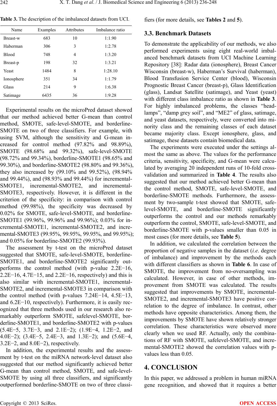

X. T. Dang et al. / J. Biomedical Science and Engineering 6 (2013) 236-248 242
Table 3. The description of the imbalanced datasets from UCI.
Name Examples Attributes Imbalance ratio
Breast-w 683 10 1:1.90
Haberman 306 3 1:2.78
Blood 748 4 1:3.20
Breast-p 198 32 1:3.21
Yeast 1484 8 1:28.10
Ionosphere 351 34 1:1.79
Glass 214 9 1:6.38
Satimage 6435 36 1:9.28
Experimental results on the microPred dataset showed
that our method achieved better G-mean than control
method, SMOTE, safe-level-SMOTE, and borderline-
SMOTE on two of three classifiers. For example, with
using SVM, although the sensitivity and G-mean in-
creased for control method (97.82% and 98.89%),
SMOTE (98.68% and 99.32%), safe-level-SMOTE
(98.72% and 99.34%), borderline-SMOTE1 (98.65% and
99.30%), and borderline-SMOTE2 (98.80% and 99.36%),
they also increased by (99.10% and 99.52%), (98.94%
and 99.44%), and (98.93% and 99.44%) for incremental-
SMOTE1, incremental-SMOTE2, and incremental-
SMOTE3, respectively. However, it is different in the
criterion of the specificity: in comparison with control
method (99.98%), the specificity was decreased by
0.02% for SMOTE, safe-level-SMOTE, and borderline-
SMOTE1 (99.96%, 99.96% and 99.96%); 0.03% for in-
cremental-SMOTE1, incremental-SMOTE2, and incre-
mental-SMOTE3 (99.95%, 99.95%, 99.95%, and 99.95%);
and 0.05% for borderline-SMOTE2 (99.93%).
The assessment by t-test on the microPred dataset
suggested that SMOTE, safe-level-SMOTE, borderline-
SMOTE1, and borderline-SMOTE2 significantly out-
performs the control method (with p-value 2.2E−16,
2.2E−16, 4.7E−15, and 2.2E−16, respectively) and this is
also similar with incremental-SMOTE1, incremental-
SMOTE2, and incremental-SMOTE3 in comparison with
the control method (with p-values 7.24E−14, 4.5E−13,
and 6.2E−10, respectively). Furthermore, it is easily rec-
ognized that three methods used in our research also re-
markably outperform SMOTE, safelevel-SMOTE, bor-
derline-SMOTE1, and borderline-SMOTE2 with p-values
(5.4E−5, 3.7E−3, and 2.1E−2); (1.9E−4, 1.2E−2, and
4.0E−2); (3.4E−5, 2.4E−3, and 1.3E−2); and (5.6E−4,
3.2E−2, and 8.0E−2), respectively.
In addition, the experimental results and the assess-
ment by t-test on the miRNA network-level dataset also
suggested that our method significantly achieved better
G-mean than control method, SMOTE, and safe-level-
SMOTE by using all three classifiers, and significantly
outperformed borderline-SMOTE on two of three classi-
fiers (for more details, see Tables 2 and 5).
3.3. Benchmark Datasets
To demonstrate the applicability of our methods, we also
performed experiments using eight real-world imbal-
anced benchmark datasets from UCI Machine Learning
Repository [38]: Radar data (ionosphere), Breast Cancer
Wisconsin (breast-w), Haberman’s Survival (haberman),
Blood Transfusion Service Center (blood), Wisconsin
Prognostic Breast Cancer (breast-p), Glass Identification
(glass), Landsat Satellite (satimage), and Yeast (yeast)
with different class imbalance ratio as shown in Table 3.
For highly imbalanced problems, the classes “head-
lamps”, “damp grey soil”, and “ME2” of glass, satimage,
and yeast datasets, respectively, were converted into mi-
nority class and the remaining classes of each dataset
became majority class. Except ionosphere, glass, and
satimage, these datasets contain biomedical data.
The experiments were executed under the settings al-
most the same as above. The values for the performance
criteria, sensitivity, specificity, and G-mean were calcu-
lated by averaging 20 independent runs of 10-fold cross-
validation and summarized in Ta bl e 4 . The results also
suggested that our method achieved better G-mean than
the control method, SMOTE, safe-level-SMOTE, and
borderline-SMOTE methods. Furthermore, the assess-
ment by two-sample t-test showed that SMOTE, safe-
level-SMOTE, and borderline-SMOTE significantly
outperforms the control and our methods remarkably
outperform the control, SMOTE, safe-level-SMOTE, and
borderline-SMOTE with p-values smaller than 0.05 in
most cases (for more details, see Table 5).
In addition, we calculated the correlation between the
proportion of negative samples in the dataset (i.e. degree
of imbalance) and improvement by the methods each
with different classifiers as shown in Ta ble 6. In case of
SMOTE, the improvement from no-oversampling was
calculated. However, in case of other methods, im-
provement from SMOTE was calculated. The results
suggested that improvements by SMOTE, incremental-
SMOTE2, and incremental-SMOTE3 have positive cor-
relation to the degree of imbalance. In contrast, other
methods have opposite characteristics. Among them, the
improvements by SMOTE have shown relatively stronger
correlation. These characteristics were observed more
clearly when we used RF. Actually, only the combina-
tions of RF with SMOTE, safelevel-SMOTE, and incre-
mental-SMOTE2 showed the correlation values with p-
values less than 0.05.
4. CONCLUSION
In this paper, we addressed a problem in human miRNA
gene recognition, and showed that it requires a better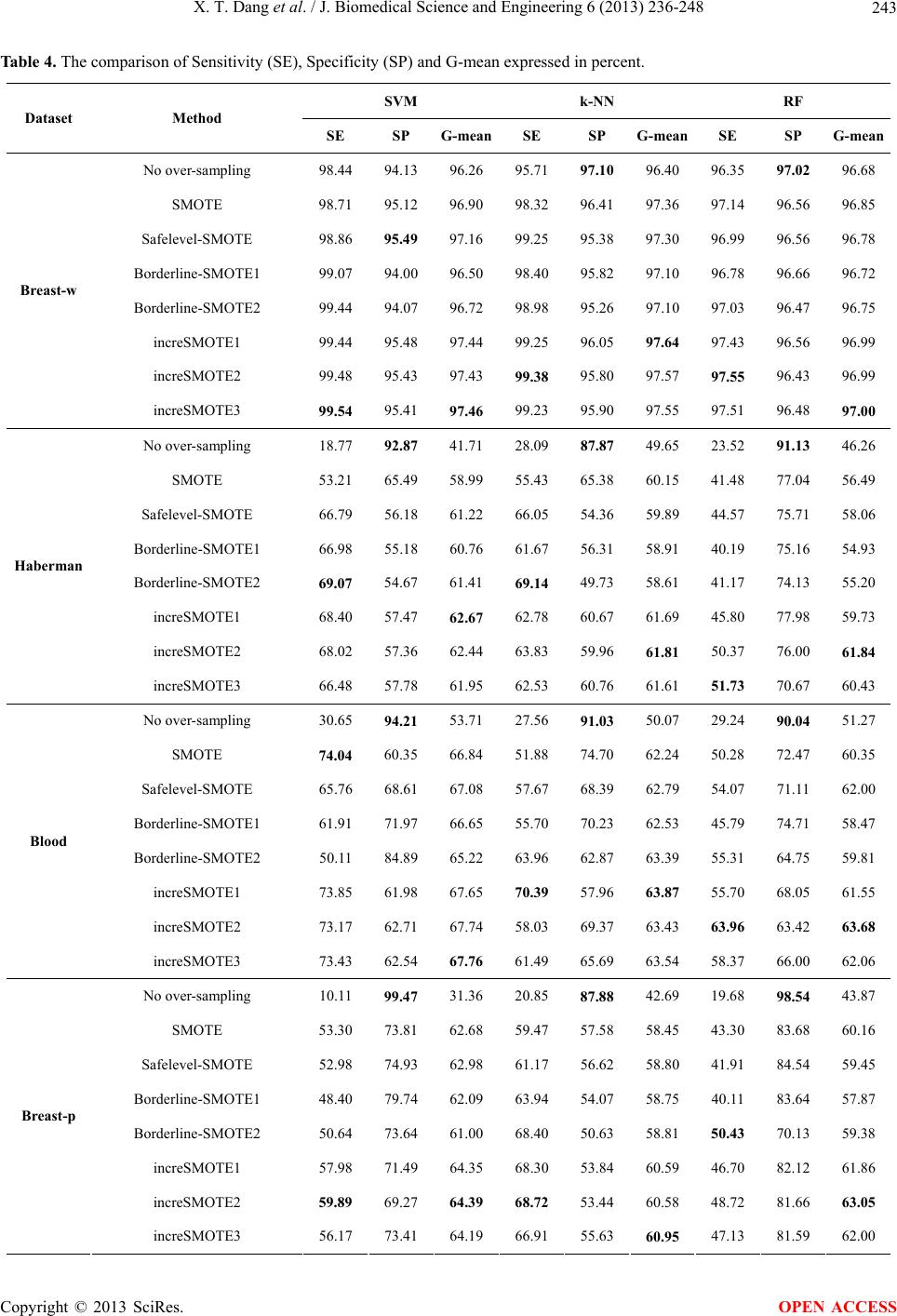

X. T. Dang et al. / J. Biomedical Science and Engineering 6 (2013) 236-248 243
Table 4. The comparison of Sensitivity (SE), Specificity (SP) and G-mean expressed in percent.
SVM k-NN RF
Dataset Method SE SP G-meanSE SP G-mean SE SP G-mean
No over-sampling 98.44 94.13 96.26 95.71 97.10 96.40 96.35 97.02 96.68
SMOTE 98.71 95.12 96.90 98.32 96.41 97.36 97.14 96.56 96.85
Safelevel-SMOTE 98.86 95.49 97.16 99.25 95.38 97.30 96.99 96.56 96.78
Borderline-SMOTE1 99.07 94.00 96.50 98.40 95.82 97.10 96.78 96.66 96.72
Borderline-SMOTE2 99.44 94.07 96.72 98.98 95.26 97.10 97.03 96.47 96.75
increSMOTE1 99.44 95.48 97.44 99.25 96.05 97.64 97.43 96.56 96.99
increSMOTE2 99.48 95.43 97.43
99.38 95.80 97.57 97.55 96.43 96.99
Breast-w
increSMOTE3 99.54 95.41 97.46 99.23 95.90 97.55 97.51 96.48 97.00
No over-sampling 18.77 92.87 41.71 28.09 87.87 49.65 23.52 91.13 46.26
SMOTE 53.21 65.49 58.99 55.43 65.38 60.15 41.48 77.04 56.49
Safelevel-SMOTE 66.79 56.18 61.22 66.05 54.36 59.89 44.57 75.71 58.06
Borderline-SMOTE1 66.98 55.18 60.76 61.67 56.31 58.91 40.19 75.16 54.93
Borderline-SMOTE2 69.07 54.67 61.41 69.14 49.73 58.61 41.17 74.13 55.20
increSMOTE1 68.40 57.47 62.67 62.78 60.67 61.69 45.80 77.98 59.73
increSMOTE2 68.02 57.36 62.44 63.83 59.96 61.81 50.37 76.00 61.84
Haberman
increSMOTE3 66.48 57.78 61.95 62.53 60.76 61.61 51.73 70.67 60.43
No over-sampling 30.65 94.21 53.71 27.56 91.03 50.07 29.24 90.04 51.27
SMOTE 74.04 60.35 66.84 51.88 74.70 62.24 50.28 72.47 60.35
Safelevel-SMOTE 65.76 68.61 67.08 57.67 68.39 62.79 54.07 71.11 62.00
Borderline-SMOTE1 61.91 71.97 66.65 55.70 70.23 62.53 45.79 74.71 58.47
Borderline-SMOTE2 50.11 84.89 65.22 63.96 62.87 63.39 55.31 64.75 59.81
increSMOTE1 73.85 61.98 67.65
70.39 57.96 63.87 55.70 68.05 61.55
increSMOTE2 73.17 62.71 67.74 58.03 69.37 63.43 63.96 63.42 63.68
Blood
increSMOTE3 73.43 62.54
67.76 61.49 65.69 63.54 58.37 66.00 62.06
No over-sampling 10.11 99.47 31.36 20.85 87.88 42.69 19.68 98.54 43.87
SMOTE 53.30 73.81 62.68 59.47 57.58 58.45 43.30 83.68 60.16
Safelevel-SMOTE 52.98 74.93 62.98 61.17 56.62 58.80 41.91 84.54 59.45
Borderline-SMOTE1 48.40 79.74 62.09 63.94 54.07 58.75 40.11 83.64 57.87
Borderline-SMOTE2 50.64 73.64 61.00 68.40 50.63 58.81 50.43 70.13 59.38
increSMOTE1 57.98 71.49 64.35 68.30 53.84 60.59 46.70 82.12 61.86
increSMOTE2 59.89 69.27 64.39 68.72 53.44 60.58 48.72 81.66 63.05
Breast-p
increSMOTE3 56.17 73.41 64.19 66.91 55.63 60.95 47.13 81.59 62.00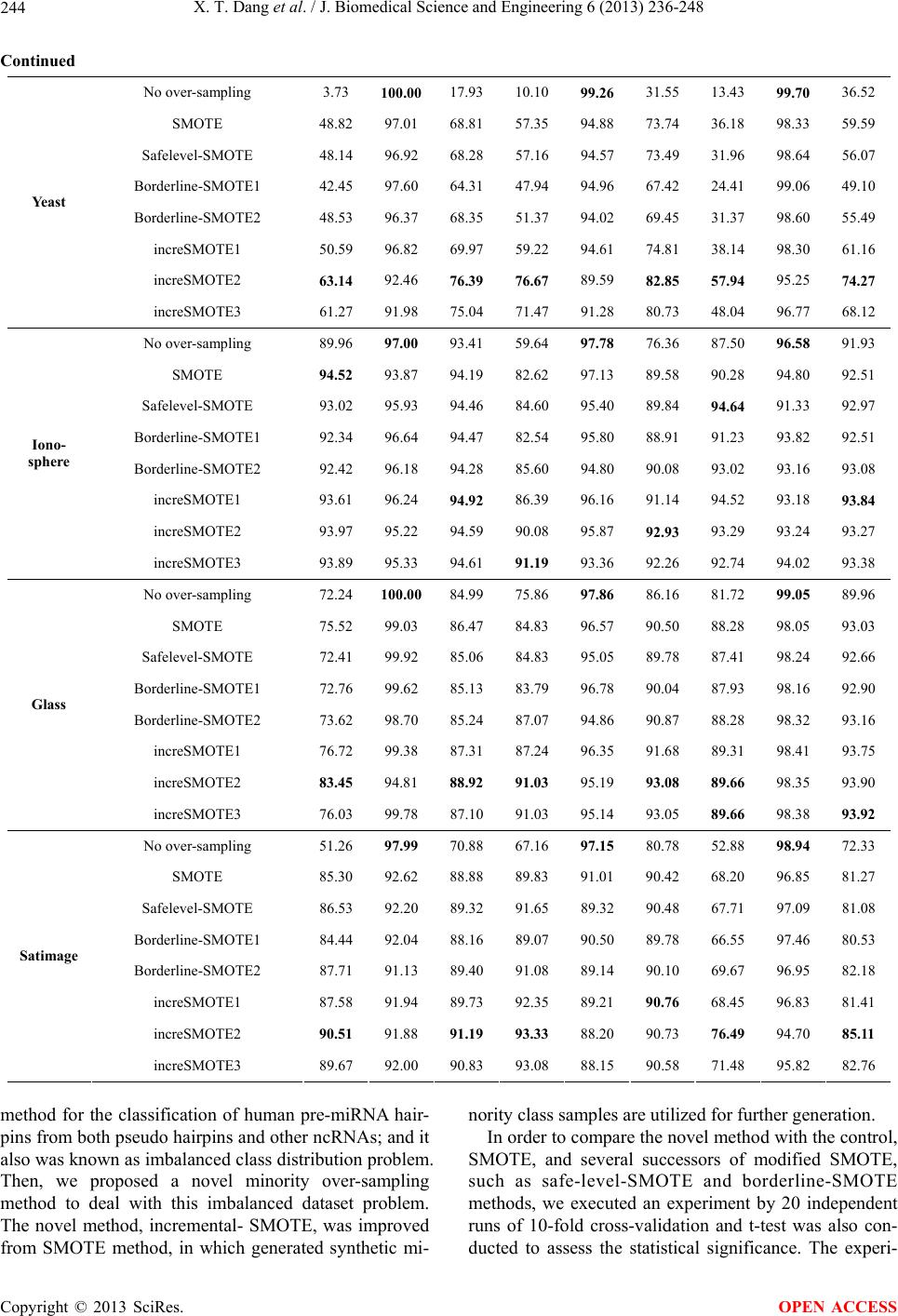

X. T. Dang et al. / J. Biomedical Science and Engineering 6 (2013) 236-248 244
Continued
No over-sampling 3.73 100.00 17.93 10.10 99.26 31.55 13.43 99.70 36.52
SMOTE 48.82 97.01 68.81 57.35 94.88 73.74 36.18 98.33 59.59
Safelevel-SMOTE 48.14 96.92 68.28 57.16 94.57 73.49 31.96 98.64 56.07
Borderline-SMOTE1 42.45 97.60 64.31 47.94 94.96 67.42 24.41 99.06 49.10
Borderline-SMOTE2 48.53 96.37 68.35 51.37 94.02 69.45 31.37 98.60 55.49
increSMOTE1 50.59 96.82 69.97 59.22 94.61 74.81 38.14 98.30 61.16
increSMOTE2 63.14 92.46 76.39 76.67 89.59 82.85 57.94 95.25 74.27
Yeast
increSMOTE3 61.27 91.98 75.04 71.47 91.28 80.73 48.04 96.77 68.12
No over-sampling 89.96 97.00 93.41 59.64 97.78 76.36 87.50 96.58 91.93
SMOTE 94.52 93.87 94.19 82.62 97.13 89.58 90.28 94.80 92.51
Safelevel-SMOTE 93.02 95.93 94.46 84.60 95.40 89.84 94.64 91.33 92.97
Borderline-SMOTE1 92.34 96.64 94.47 82.54 95.80 88.91 91.23 93.82 92.51
Borderline-SMOTE2 92.42 96.18 94.28 85.60 94.80 90.08 93.02 93.16 93.08
increSMOTE1 93.61 96.24 94.92 86.39 96.16 91.14 94.52 93.18 93.84
increSMOTE2 93.97 95.22 94.59 90.08 95.87 92.93 93.29 93.24 93.27
Iono-
sphere
increSMOTE3 93.89 95.33 94.61 91.19 93.36 92.26 92.74 94.02 93.38
No over-sampling 72.24 100.00 84.99 75.86 97.86 86.16 81.72 99.05 89.96
SMOTE 75.52 99.03 86.47 84.83 96.57 90.50 88.28 98.05 93.03
Safelevel-SMOTE 72.41 99.92 85.06 84.83 95.05 89.78 87.41 98.24 92.66
Borderline-SMOTE1 72.76 99.62 85.13 83.79 96.78 90.04 87.93 98.16 92.90
Borderline-SMOTE2 73.62 98.70 85.24 87.07 94.86 90.87 88.28 98.32 93.16
increSMOTE1 76.72 99.38 87.31 87.24 96.35 91.68 89.31 98.41 93.75
increSMOTE2 83.45 94.81 88.92 91.03 95.19 93.08 89.66 98.35 93.90
Glass
increSMOTE3 76.03 99.78 87.10 91.03 95.14 93.05 89.66 98.38 93.92
No over-sampling 51.26 97.99 70.88 67.16 97.15 80.78 52.88 98.94 72.33
SMOTE 85.30 92.62 88.88 89.83 91.01 90.42 68.20 96.85 81.27
Safelevel-SMOTE 86.53 92.20 89.32 91.65 89.32 90.48 67.71 97.09 81.08
Borderline-SMOTE1 84.44 92.04 88.16 89.07 90.50 89.78 66.55 97.46 80.53
Borderline-SMOTE2 87.71 91.13 89.40 91.08 89.14 90.10 69.67 96.95 82.18
increSMOTE1 87.58 91.94 89.73 92.35 89.21 90.76 68.45 96.83 81.41
increSMOTE2 90.51 91.88 91.19 93.33 88.20 90.73 76.49 94.70 85.11
Satimage
increSMOTE3 89.67 92.00 90.83 93.08 88.15 90.58 71.48 95.82 82.76
method for the classification of human pre-miRNA hair-
pins from both pseudo hairpins and other ncRNAs; and it
also was known as imbalanced class distribution problem.
Then, we proposed a novel minority over-sampling
method to deal with this imbalanced dataset problem.
The novel method, incremental- SMOTE, was improved
from SMOTE method, in which generated synthetic mi-
nority class samples are utilized for further generation.
In order to compare the novel method with the control,
SMOTE, and several successors of modified SMOTE,
such as safe-level-SMOTE and borderline-SMOTE
methods, we executed an experiment by 20 independent
runs of 10-fold cross-validation and t-test was also con-
ducted to assess the statistical significance. The experi-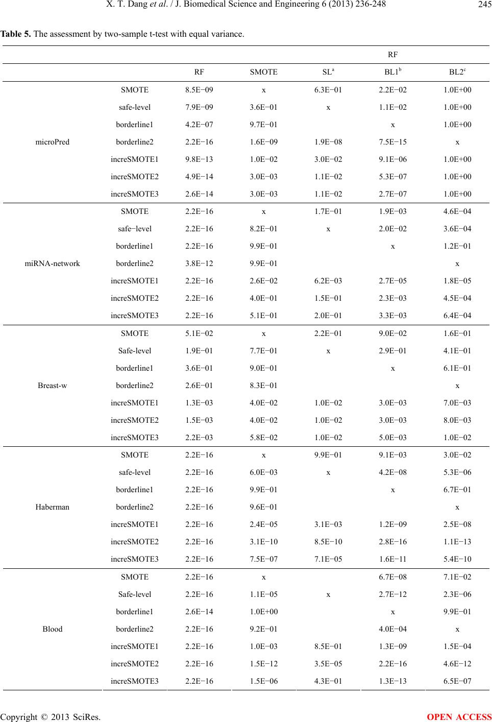

X. T. Dang et al. / J. Biomedical Science and Engineering 6 (2013) 236-248 245
Table 5. The assessment by two-sample t-test with equal variance.
RF
RF SMOTE SLa BL1b BL2c
SMOTE 8.5E−09 x 6.3E−01 2.2E−02 1.0E+00
safe-level 7.9E−09 3.6E−01 x 1.1E−02 1.0E+00
borderline1 4.2E−07 9.7E−01 x 1.0E+00
borderline2 2.2E−16 1.6E−09 1.9E−08 7.5E−15 x
increSMOTE1 9.8E−13 1.0E−02 3.0E−02 9.1E−06 1.0E+00
increSMOTE2 4.9E−14 3.0E−03 1.1E−02 5.3E−07 1.0E+00
microPred
increSMOTE3 2.6E−14 3.0E−03 1.1E−02 2.7E−07 1.0E+00
SMOTE 2.2E−16 x 1.7E−01 1.9E−03 4.6E−04
safe−level 2.2E−16 8.2E−01 x 2.0E−02 3.6E−04
borderline1 2.2E−16 9.9E−01 x 1.2E−01
borderline2 3.8E−12 9.9E−01 x
increSMOTE1 2.2E−16 2.6E−02 6.2E−03 2.7E−05 1.8E−05
increSMOTE2 2.2E−16 4.0E−01 1.5E−01 2.3E−03 4.5E−04
miRNA-network
increSMOTE3 2.2E−16 5.1E−01 2.0E−01 3.3E−03 6.4E−04
SMOTE 5.1E−02 x 2.2E−01 9.0E−02 1.6E−01
Safe-level 1.9E−01 7.7E−01 x 2.9E−01 4.1E−01
borderline1 3.6E−01 9.0E−01 x 6.1E−01
borderline2 2.6E−01 8.3E−01 x
increSMOTE1 1.3E−03 4.0E−02 1.0E−02 3.0E−03 7.0E−03
increSMOTE2 1.5E−03 4.0E−02 1.0E−02 3.0E−03 8.0E−03
Breast-w
increSMOTE3 2.2E−03 5.8E−02 1.0E−02 5.0E−03 1.0E−02
SMOTE 2.2E−16 x 9.9E−01 9.1E−03 3.0E−02
safe-level 2.2E−16 6.0E−03 x 4.2E−08 5.3E−06
borderline1 2.2E−16 9.9E−01 x 6.7E−01
borderline2 2.2E−16 9.6E−01 x
increSMOTE1 2.2E−16 2.4E−05 3.1E−03 1.2E−09 2.5E−08
increSMOTE2 2.2E−16 3.1E−10 8.5E−10 2.8E−16 1.1E−13
Haberman
increSMOTE3 2.2E−16 7.5E−07 7.1E−05 1.6E−11 5.4E−10
SMOTE 2.2E−16 x 6.7E−08 7.1E−02
Safe-level 2.2E−16 1.1E−05 x 2.7E−12 2.3E−06
borderline1 2.6E−14 1.0E+00 x 9.9E−01
borderline2 2.2E−16 9.2E−01 4.0E−04 x
increSMOTE1 2.2E−16 1.0E−03 8.5E−01 1.3E−09 1.5E−04
increSMOTE2 2.2E−16 1.5E−12 3.5E−05 2.2E−16 4.6E−12
Blood
increSMOTE3 2.2E−16 1.5E−06 4.3E−01 1.3E−13 6.5E−07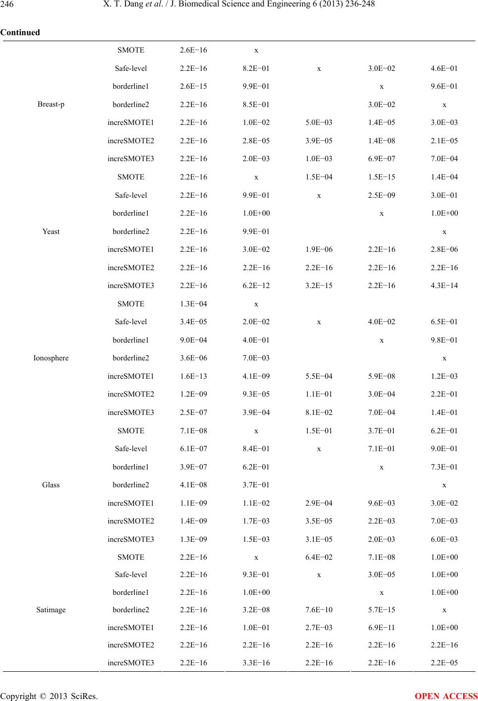

X. T. Dang et al. / J. Biomedical Science and Engineering 6 (2013) 236-248 246
Continued
SMOTE 2.6E−16 x
Safe-level 2.2E−16 8.2E−01 x 3.0E−02 4.6E−01
borderline1 2.6E−15 9.9E−01 x 9.6E−01
borderline2 2.2E−16 8.5E−01 3.0E−02 x
increSMOTE1 2.2E−16 1.0E−02 5.0E−03 1.4E−05 3.0E−03
increSMOTE2 2.2E−16 2.8E−05 3.9E−05 1.4E−08 2.1E−05
Breast-p
increSMOTE3 2.2E−16 2.0E−03 1.0E−03 6.9E−07 7.0E−04
SMOTE 2.2E−16 x 1.5E−04 1.5E−15 1.4E−04
Safe-level 2.2E−16 9.9E−01 x 2.5E−09 3.0E−01
borderline1 2.2E−16 1.0E+00 x 1.0E+00
borderline2 2.2E−16 9.9E−01 x
increSMOTE1 2.2E−16 3.0E−02 1.9E−06 2.2E−16 2.8E−06
increSMOTE2 2.2E−16 2.2E−16 2.2E−16 2.2E−16 2.2E−16
Yeast
increSMOTE3 2.2E−16 6.2E−12 3.2E−15 2.2E−16 4.3E−14
SMOTE 1.3E−04 x
Safe-level 3.4E−05 2.0E−02 x 4.0E−02 6.5E−01
borderline1 9.0E−04 4.0E−01 x 9.8E−01
borderline2 3.6E−06 7.0E−03 x
increSMOTE1 1.6E−13 4.1E−09 5.5E−04 5.9E−08 1.2E−03
increSMOTE2 1.2E−09 9.3E−05 1.1E−01 3.0E−04 2.2E−01
Ionosphere
increSMOTE3 2.5E−07 3.9E−04 8.1E−02 7.0E−04 1.4E−01
SMOTE 7.1E−08 x 1.5E−01 3.7E−01 6.2E−01
Safe-level 6.1E−07 8.4E−01 x 7.1E−01 9.0E−01
borderline1 3.9E−07 6.2E−01 x 7.3E−01
borderline2 4.1E−08 3.7E−01 x
increSMOTE1 1.1E−09 1.1E−02 2.9E−04 9.6E−03 3.0E−02
increSMOTE2 1.4E−09 1.7E−03 3.5E−05 2.2E−03 7.0E−03
Glass
increSMOTE3 1.3E−09 1.5E−03 3.1E−05 2.0E−03 6.0E−03
SMOTE 2.2E−16 x 6.4E−02 7.1E−08 1.0E+00
Safe-level 2.2E−16 9.3E−01 x 3.0E−05 1.0E+00
borderline1 2.2E−16 1.0E+00 x 1.0E+00
borderline2 2.2E−16 3.2E−08 7.6E−10 5.7E−15 x
increSMOTE1 2.2E−16 1.0E−01 2.7E−03 6.9E−11 1.0E+00
increSMOTE2 2.2E−16 2.2E−16 2.2E−16 2.2E−16 2.2E−16
Satimage
increSMOTE3 2.2E−16 3.3E−16 2.2E−16 2.2E−16 2.2E−05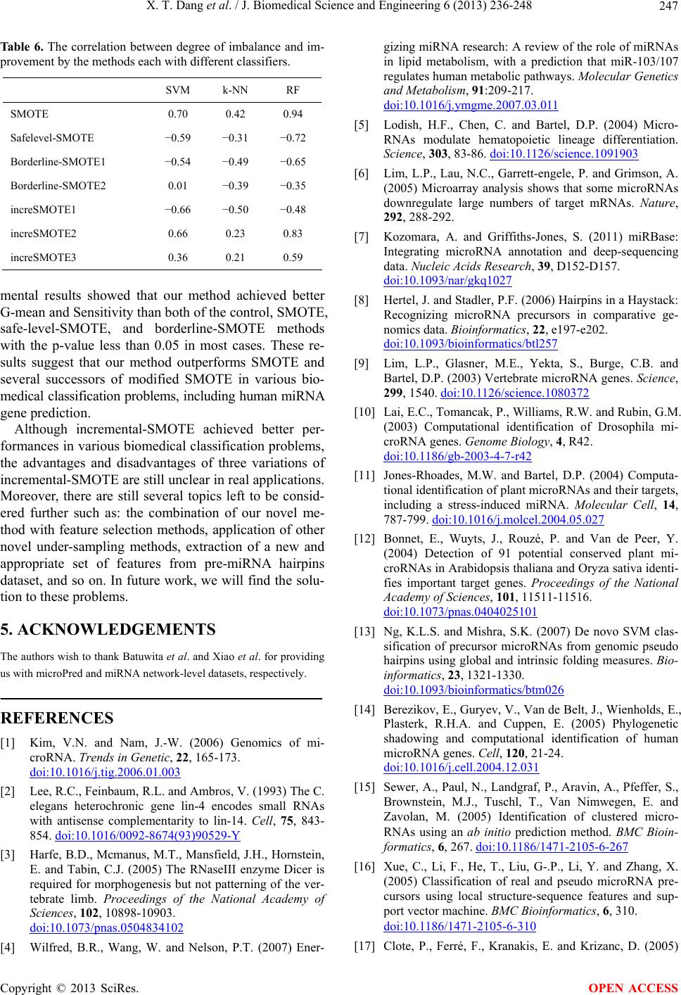

X. T. Dang et al. / J. Biomedical Science and Engineering 6 (2013) 236-248 247
Ta bl e 6. The correlation between degree of imbalance and im-
provement by the methods each with different classifiers.
SVM k-NN RF
SMOTE 0.70 0.42 0.94
Safelevel-SMOTE −0.59 −0.31 −0.72
Borderline-SMOTE1 −0.54 −0.49 −0.65
Borderline-SMOTE2 0.01 −0.39 −0.35
increSMOTE1 −0.66 −0.50 −0.48
increSMOTE2 0.66 0.23 0.83
increSMOTE3 0.36 0.21 0.59
mental results showed that our method achieved better
G-mean and Sensitivity than both of the control, SMOTE,
safe-level-SMOTE, and borderline-SMOTE methods
with the p-value less than 0.05 in most cases. These re-
sults suggest that our method outperforms SMOTE and
several successors of modified SMOTE in various bio-
medical classification problems, including human miRNA
gene prediction.
Although incremental-SMOTE achieved better per-
formances in various biomedical classification problems,
the advantages and disadvantages of three variations of
incremental-SMOTE are still unclear in real applications.
Moreover, there are still several topics left to be consid-
ered further such as: the combination of our novel me-
thod with feature selection methods, application of other
novel under-sampling methods, extraction of a new and
appropriate set of features from pre-miRNA hairpins
dataset, and so on. In future work, we will find the solu-
tion to these problems.
5. ACKNOWLEDGEMENTS
The authors wish to thank Batuwita et al. and Xiao et al. for providing
us with microPred and miRNA network-level datasets, respectively.
REFERENCES
[1] Kim, V.N. and Nam, J.-W. (2006) Genomics of mi-
croRNA. Trends in Genetic, 22, 165-173.
doi:10.1016/j.tig.2006.01.003
[2] Lee, R.C., Feinbaum, R.L. and Ambros, V. (1993) The C.
elegans heterochronic gene lin-4 encodes small RNAs
with antisense complementarity to lin-14. Cell, 75, 843-
854. doi:10.1016/0092-8674(93)90529-Y
[3] Harfe, B.D., Mcmanus, M.T., Mansfield, J.H., Hornstein,
E. and Tabin, C.J. (2005) The RNaseIII enzyme Dicer is
required for morphogenesis but not patterning of the ver-
tebrate limb. Proceedings of the National Academy of
Sciences, 102, 10898-10903.
doi:10.1073/pnas.0504834102
[4] Wilfred, B.R., Wang, W. and Nelson, P.T. (2007) Ener-
gizing miRNA research: A review of the role of miRNAs
in lipid metabolism, with a prediction that miR-103/107
regulates human metabolic pathways. Molecular Genetics
and Metabolism, 91:209-217.
doi:10.1016/j.ymgme.2007.03.011
[5] Lodish, H.F., Chen, C. and Bartel, D.P. (2004) Micro-
RNAs modulate hematopoietic lineage differentiation.
Science, 303, 83-86. doi:10.1126/science.1091903
[6] Lim, L.P., Lau, N.C., Garrett-engele, P. and Grimson, A.
(2005) Microarray analysis shows that some microRNAs
downregulate large numbers of target mRNAs. Nature,
292, 288-292.
[7] Kozomara, A. and Griffiths-Jones, S. (2011) miRBase:
Integrating microRNA annotation and deep-sequencing
data. Nucleic Acids Rese arch, 39, D152-D157.
doi:10.1093/nar/gkq1027
[8] Hertel, J. and Stadler, P.F. (2006) Hairpins in a Haystack:
Recognizing microRNA precursors in comparative ge-
nomics data. Bioinformatics, 22, e197-e202.
doi:10.1093/bioinformatics/btl257
[9] Lim, L.P., Glasner, M.E., Yekta, S., Burge, C.B. and
Bartel, D.P. (2003) Vertebrate microRNA genes. Science,
299, 1540. doi:10.1126/science.1080372
[10] Lai, E.C., Tomancak, P., Williams, R.W. and Rubin, G.M.
(2003) Computational identification of Drosophila mi-
croRNA genes. Genome Biology, 4, R42.
doi:10.1186/gb-2003-4-7-r42
[11] Jones-Rhoades, M.W. and Bartel, D.P. (2004) Computa-
tional identification of plant microRNAs and their targets,
including a stress-induced miRNA. Molecular Cell, 14,
787-799. doi:10.1016/j.molcel.2004.05.027
[12] Bonnet, E., Wuyts, J., Rouzé, P. and Van de Peer, Y.
(2004) Detection of 91 potential conserved plant mi-
croRNAs in Arabidopsis thaliana and Oryza sativa identi-
fies important target genes. Proceedings of the National
Academy of Sciences, 101, 11511-11516.
doi:10.1073/pnas.0404025101
[13] Ng, K.L.S. and Mishra, S.K. (2007) De novo SVM clas-
sification of precursor microRNAs from genomic pseudo
hairpins using global and intrinsic folding measures. Bio-
informatics, 23, 1321-1330.
doi:10.1093/bioinformatics/btm026
[14] Berezikov, E., Guryev, V., Van de Belt, J., Wienholds, E.,
Plasterk, R.H.A. and Cuppen, E. (2005) Phylogenetic
shadowing and computational identification of human
microRNA genes. Cell, 120, 21-24.
doi:10.1016/j.cell.2004.12.031
[15] Sewer, A., Paul, N., Landgraf, P., Aravin, A., Pfeffer, S.,
Brownstein, M.J., Tuschl, T., Van Nimwegen, E. and
Zavolan, M. (2005) Identification of clustered micro-
RNAs using an ab initio prediction method. BMC Bioin-
formatics, 6, 267. doi:10.1186/1471-2105-6-267
[16] Xue, C., Li, F., He, T., Liu, G-.P., Li, Y. and Zhang, X.
(2005) Classification of real and pseudo microRNA pre-
cursors using local structure-sequence features and sup-
port vector machine. BMC Bioinformatics, 6, 310.
doi:10.1186/1471-2105-6-310
[17] Clote, P., Ferré, F., Kranakis, E. and Krizanc, D. (2005)

X. T. Dang et al. / J. Biomedical Science and Engineering 6 (2013) 236-248 248
Structural RNA has lower folding energy than random
RNA of the same dinucleotide frequency. RNA, 11, 578-
591. doi:10.1261/rna.7220505
[18] Jiang, P., Wu, H., Wang, W., Ma, W., Sun, X. and Lu, Z.
(2007) MiPred: Classification of real and pseudo micro-
RNA precursors using random forest prediction model
with combined features. Nucleic Acids Re search, 35, 339-
344. doi:10.1093/nar/gkm368
[19] Tang, X., Xiao, J., Li, Y., Wen, Z., Fang, Z. and Li, M.
(2012) Systematic analysis revealed better performance
of random forest algorithm coupled with complex net-
work features in predicting microRNA precursors. Che-
mometrics and Intelligent Laboratory Systems, 118, 317-
323. doi:10.1016/j.chemolab.2012.05.001
[20] Wang, Y., Chen, X., Jiang, W., Li, L., Li, W., Yang, L.,
Liao, M., Lian, B., Lv, Y., Wang, S., Wang, S. and Li, X.
(2011) Predicting human microRNA precursors based on
an optimized feature subset generated by GA-SVM. Ge-
nomics, 98, 73-78. doi:10.1016/j.ygeno.2011.04.011
[21] Zhang, Y., Yang, Y., Zhang, H., Jiang, X., Xu, B., Xue,
Y., Cao, Y., Zhai, Q., Zhai, Y., Xu, M., Cooke, H.J. and
Shi, Q. (2011) Prediction of novel pre-microRNAs with
high accuracy through boosting and SVM. Bioinformatics,
27, 1436-1437. doi:10.1093/bioinformatics/btr148
[22] Kadri, S., Hinman, V. and Benos, P.V. (2009) HHMMiR:
Efficient de novo prediction of microRNAs using hierar-
chical hidden Markov models. BMC Bioinformatics, 10,
S35. doi:10.1186/1471-2105-10-S1-S35
[23] Batuwita, R. and Palade, V. (2009) microPred: Effective
classification of pre-miRNAs for human miRNA gene
prediction. Bioinformatics, 25, 989-995.
doi:10.1093/bioinformatics/btp107
[24] Xiao, J., Tang, X., Li, Y., Fang, Z., Ma, D., He, Y. and Li,
M. (2011) Identification of microRNA precursors based
on random forest with network-level representation me-
thod of stem-loop structure. BMC Bioinformatics, 12, 165.
doi:10.1186/1471-2105-12-165
[25] Bunkhumpornpat, C., Sinapiromsaran, K. and Lursinsap,
C. (2009) Safe-Level-SMOTE: Safe-level-synthetic mi-
nority over-sampling technique. Lecture Notes in Com-
puter Science, 5476, 475-482.
doi:10.1007/978-3-642-01307-2_43
[26] Han, H., Wang, W. and Mao, B. (2005) Borderline-
SMOTE: A new over-sampling method in imbalanced
data sets learning. Lecture Notes in Computer Science,
3644, 878-887. doi:10.1007/11538059_91
[27] Chawla, N.V., Bowyer, K.W. and Hall, L.O. (2002)
SMOTE : Synthetic minority over-sampling technique.
Journal of Artificial Intelligence Research, 16, 321-357.
[28] Burges, C.J.C. (1998) A tutorial on support vector ma-
chines for pattern recognition. Data Mining and Knowl-
edge Discovery, 2, 121-167.
doi:10.1023/A:1009715923555
[29] Vapnik, V.N. (1999) An overview of statistical learning
theory. IEEE Transactions on Neural networks, 10, 988-
999. doi:10.1109/72.788640
[30] Karatzoglou, A. and Smola, A. (2004) kernlab—An S4
package for kernel methods in R. Journal of Statistical
Software, 11, 1-20.
[31] Venables, W.N. and Ripley, B.D. (2002) Modern applied
statistics with S. 4th Edition. Springer, New York.
doi:10.1007/978-0-387-21706-2
[32] Liaw, A. and Wiener, M. (2002) Classification and re-
gression by random forest. R News, 2, 18-22.
[33] Akbani, R., Kwek, S. and Japkowicz, N. (2004) Applying
support vector machines to imbalanced datasets. Lecture
Notes in Computer Science, 3201, 39-50.
doi:10.1007/978-3-540-30115-8_7
[34] Anand, A., Pugalenthi, G., Fogel, G.B. and Suganthan,
P.N. (2010) An approach for classification of highly im-
balanced data using weighting and undersampling. Amino
Acids, 39, 1385-1391. doi:10.1007/s00726-010-0595-2
[35] Kubat, M. and Matwin, S. (8-12 July 1997) Addressing
the curse of imbalanced training sets: One-sided selection.
Proceedings of the 14th International Conference in Ma-
chine Learning, Nashville, 179-186.
[36] Han, K. (2011) Effective sample selection for classifica-
tion of pre-miRNAs. Genetics and Molecular Research,
10, 506-518. doi:10.4238/vol10-1gmr1054
[37] Xuan, P., Guo, M., Liu, X., Huang, Y., Li, W. and Huang,
Y. (2011) PlantMiRNAPred: Efficient classification of
real and pseudo plant pre-miRNAs. Bioinformatics, 27,
1368-1376. doi:10.1093/bioinformatics/btr153
[38] Frank, A. and Asuncion, A. (2010) UCI machine learning
repository. University of California, Irvine.