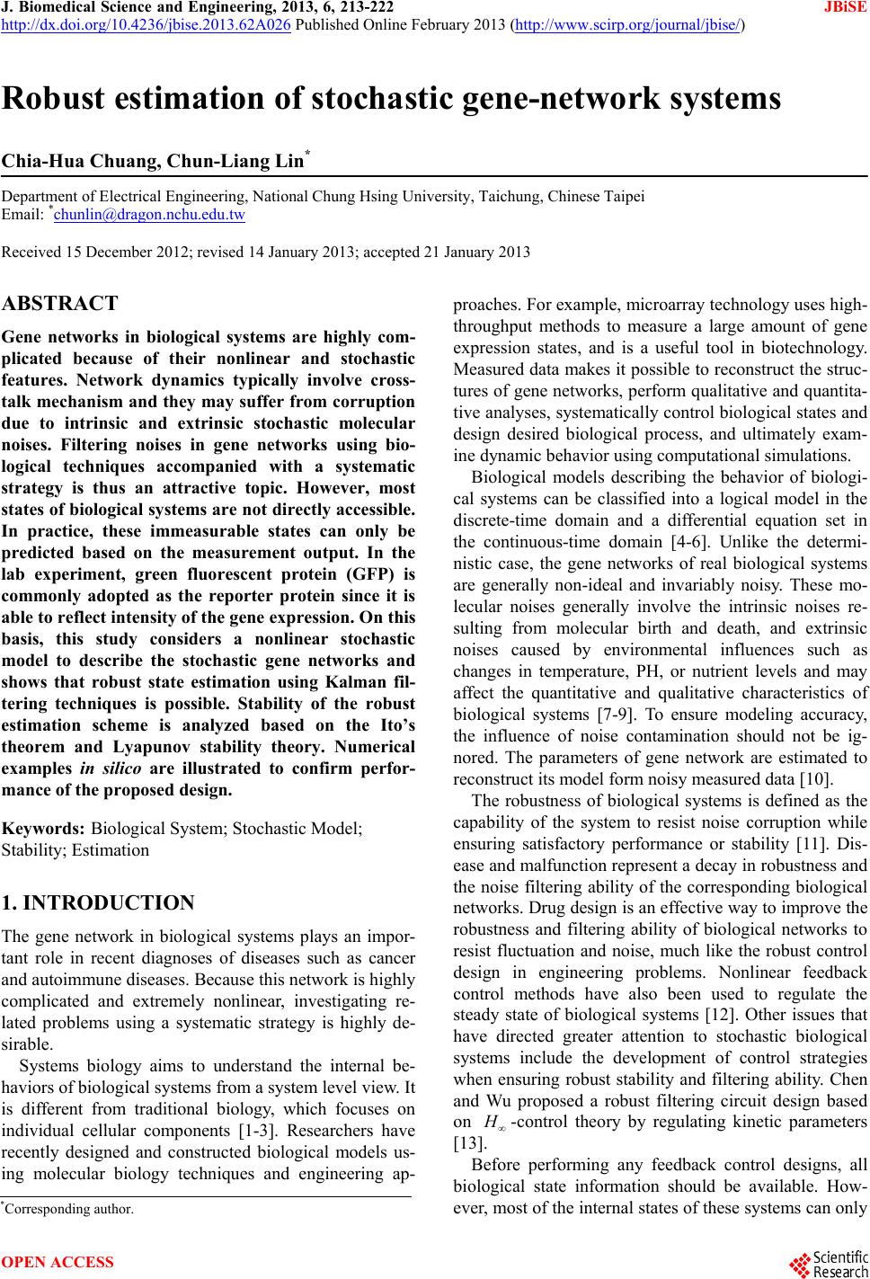
 J. Biomedical Science and Engineering, 2013, 6, 213-222 JBiSE http://dx.doi.org/10.4236/jbise.2013.62A026 Published Online February 2013 (http://www.scirp.org/journal/jbise/) Robust estimation of stochastic gene-network systems Chia-Hua Chuang, Chun-Liang Lin* Department of Electrical Engineering, National Chung Hsing University, Taichung, Chinese Taipei Email: *chunlin@dragon.nchu.edu.tw Received 15 December 2012; revised 14 January 2013; accepted 21 January 2013 ABSTRACT Gene networks in biological systems are highly com- plicated because of their nonlinear and stochastic features. Network dynamics typically involve cross- talk mechanism and they may suffer from corruption due to intrinsic and extrinsic stochastic molecular noises. Filtering noises in gene networks using bio- logical techniques accompanied with a systematic strategy is thus an attractive topic. However, most states of biological systems are not directly accessible. In practice, these immeasurable states can only be predicted based on the measurement output. In the lab experiment, green fluorescent protein (GFP) is commonly adopted as the reporter protein since it is able to reflect intensity of the gene expression. On this basis, this study considers a nonlinear stochastic model to describe the stochastic gene networks and shows that robust state estimation using Kalman fil- tering techniques is possible. Stability of the robust estimation scheme is analyzed based on the Ito’s theorem and Lyapunov stability theory. Numerical examples in silico are illustrated to confirm perfor- mance of the proposed design. Keywords: Biological System; Stochastic Model; Stability; Estimation 1. INTRODUCTION The gene network in biological systems plays an impor- tant role in recent diagnoses of diseases such as cancer and autoimmune diseases. Because this network is highly complicated and extremely nonlinear, investigating re- lated problems using a systematic strategy is highly de- sirable. Systems biology aims to understand the internal be- haviors of biological systems from a system level view. It is different from traditional biology, which focuses on individual cellular components [1-3]. Researchers have recently designed and constructed biological models us- ing molecular biology techniques and engineering ap- proaches. For example, microarray technology uses high- throughput methods to measure a large amount of gene expression states, and is a useful tool in biotechnology. Measured data makes it possible to reconstruct the struc- tures of gene networks, perform qualitative an d quantita- tive analyses, systematically control biological states and design desired biological process, and ultimately exam- ine dynamic behavior using computational simulations. Biological models describing the behavior of biologi- cal systems can be classified into a logical model in the discrete-time domain and a differential equation set in the continuous-time domain [4-6]. Unlike the determi- nistic case, the gene networks of real biological systems are generally non-ideal and invariably noisy. These mo- lecular noises generally involve the intrinsic noises re- sulting from molecular birth and death, and extrinsic noises caused by environmental influences such as changes in temperature, PH, or nutrient levels and may affect the quantitative and qualitative characteristics of biological systems [7-9]. To ensure modeling accuracy, the influence of noise contamination should not be ig- nored. The parameters of gene network are estimated to reconstruct its model form noisy measured data [10]. The robustness of biological systems is defined as the capability of the system to resist noise corruption while ensuring satisfactory performance or stability [11]. Dis- ease and malfunction represent a decay in robustness and the noise filtering ability of the corresponding biological networks. Drug design is an effective way to improve the robustness and filtering ability of biological networks to resist fluctuation and noise, much like the robust control design in engineering problems. Nonlinear feedback control methods have also been used to regulate the steady state of biological systems [12]. Other issues that have directed greater attention to stochastic biological systems include the development of control strategies when ensuring robust stability and filtering ability. Chen and Wu proposed a robust filtering circuit design based on -control theory by regulating kinetic parameters [13]. Before performing any feedback control designs, all biological state information should be available. How- ever, most of the internal states of these systems can only *Corresponding author. OPEN ACCESS 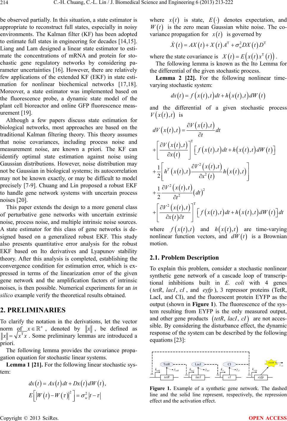 C.-H. Chuang, C.-L. Lin / J. Biomedical Science and Engineering 6 (2013) 213-222 214 be observed partially. In this situation, a state estimator is appropriate to reconstruct full states, especially in noisy environments. The Kalman filter (KF) has been adopted to estimate full states in engineering for decades [14,15]. Liang and Lam designed a linear state estimator to esti- mate the concentrations of mRNA and protein for sto- chastic gene regulatory networks by considering pa- rameter uncertainties [16]. However, there are relatively few applications of the extended KF (EKF) in state esti- mation for nonlinear biochemical networks [17,18]. Moreover, a state estimator was implemented based on the fluorescence probe, a dynamic state model of the plant cell bioreactor and online GFP fluorescence meas- urement [19]. Although a few papers discuss state estimation for biological networks, most approaches are based on the traditional Kalman filtering theory. This theory assumes that noise covariances, including process noise and measurement noise, are known a priori. The KF can identify optimal state estimation against noise using Gaussian distributions. However, noise distribution may not be Gaussian in b iological systems; its autocorrelation may not be known exactly, or may be difficult to model precisely [7-9]. Chuang and Lin proposed a robust EKF to handle gene network systems with uncertain process noises [20]. This paper extends the design to a more general class of perturbative gene networks with uncertain extrinsic noise, process noise, and multiple in trinsic noise sources. A state estimator for this class of gene networks is de- signed based on a generalized robust EKF. This study also presents quantitative error analysis for the robust EKF based on Ito derivatives and Lyapunov stability theory. After this analysis is completed, establishing the convergence condition for estimation error, which is ex- pressed in terms of the linearization error of the given gene network and the amplification factors of intrinsic noises, is then possible. Numerical experiments for an in silico example verify the theoretical results obtained. 2. PRELIMINARIES To clarify the notation in the derivations, let the vector norm of , denoted by n x , be defined as T xx. Some preliminary lemmas are introduced a priori. The following lemma provides the covariance propa- gation equation for stochastic linear systems. Lemma 1 [21]. For the following linear stochastic sys- tem: 22 , w dx tAx tdtDx tdWt EWt Wt where t is state, E denotes expectation, and Wt is the zero mean Gaussian white noise. The co- variance propa gati on for t is governe d by T2 w T tAXt XtADXtD where the state covariance is T tExtxt. The following lemma is known as the Ito Lemma for the differential of the given stochastic process. Lemma 2 [22]. For the following nonlinear time- varying stochastic system: ,,dxtfxt tdthxttdWt and the differential of a given stochastic process ,Vxtt is T 2 2 22 2 T 2 , , ,,, , 1,, 2 , 1 2 ,,, T Vxt t dVx ttdt t Vxttfxttdth xtt dWt xt Vxtt h xtthxtt xt Vxttdt t Vxtt xt tdthxttdWtdt xt t where , xt t and are time-varying nonlinear function vectors, and is a Brownian motion. ,hxt t dW t 2.1. Problem Description To explain this problem, consider a stochastic nonlinear synthetic gene network of a cascade loop of transcrip- tional inhibitions built in E. coli with 4 genes (, and ), 3 repressor proteins (TetR, LacI, and CI), and the fluorescent protein EYFP as the output (shown in Figure 1). The fluorescence of the sys- tem resulting from EYFP is the only measured output, and other gene products , , tetR lacIcIeyfp , , tetR lacIcI are not acces- sible. By considering the disturbance effect, the dynamic response of the system can be described by the following equations [23]: tetR lacI cI eyfp TetR LacI CI EYFP tetR eyfp lacl cl lacl keyfp k cl k tetR k Figure 1. Example of a synthetic gene network. The dashed line and the solid line represent, respectively, the repression effect and the activation effect. Copyright © 2013 SciRes. OPEN ACCESS 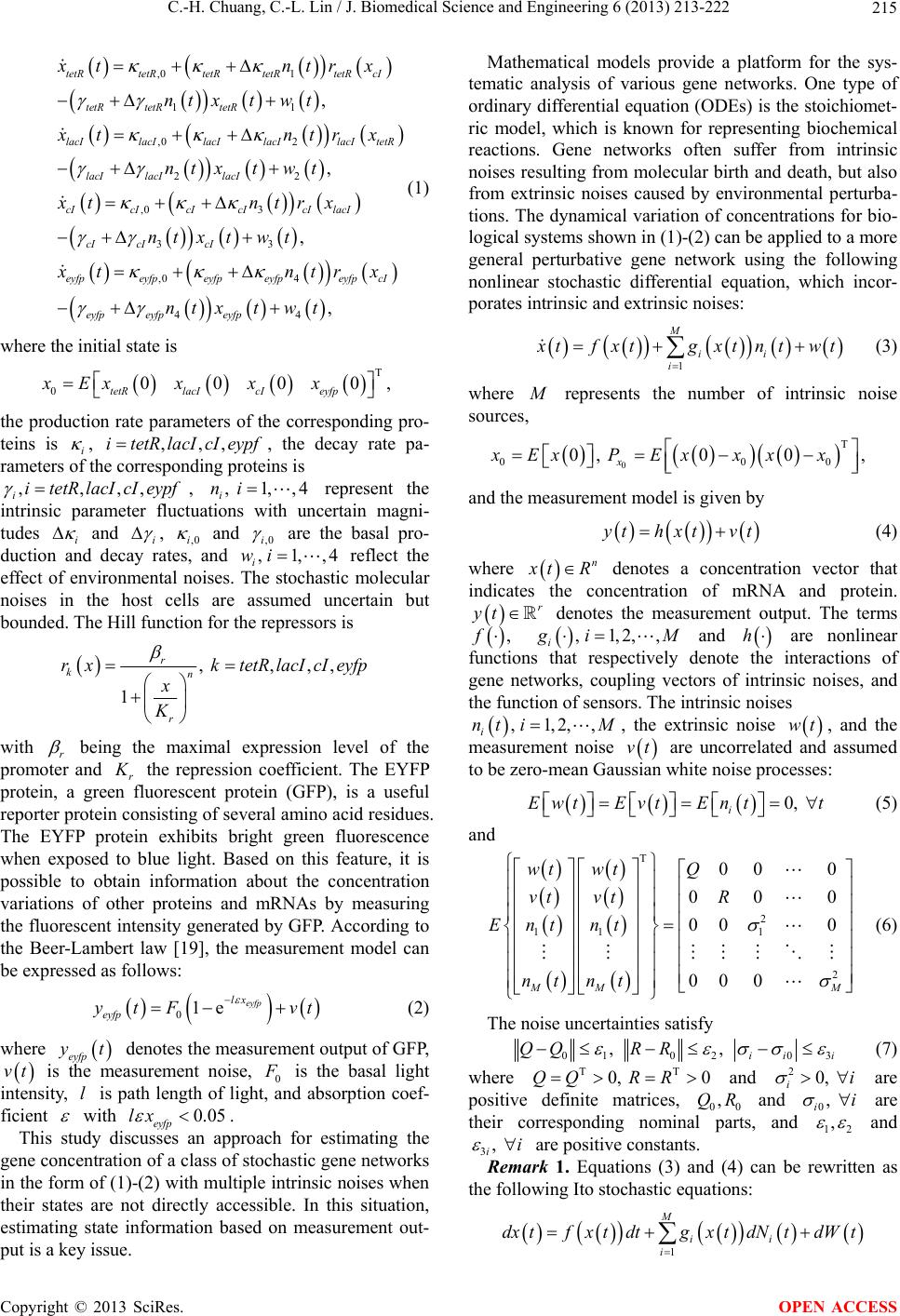 C.-H. Chuang, C.-L. Lin / J. Biomedical Science and Engineering 6 (2013) 213-222 215 ,0 1 11 ,0 2 22 ,0 3 33 , , , , tetRtetRtetRtetRtetR cI tetR tetRtetR lacIlacIlacIlacIlacI tetR lacI lacIlacI cIcIcIcIcI lacI cI cIcI eyfp eyfp xt ntrx nt xtwt xt ntrx ntxt wt xt ntrx ntxtwt xt 04 44 , eyfpeyfpeyfp cI eyfp eyfpeyfp ntr x ntxt wt (1) where the initial state is T 00000 tetR lacIcIeyfp xExxxx , the production rate parameters of the corresponding pro- teins is i, , the decay rate pa- rameters of the corresponding proteins is ,,,itetR lacIcIeypf ,,,, iitetRlacI cI eypf , represent the intrinsic parameter fluctuations with uncertain magni- tudes i and i , 1,,4 i ni , ,0i and ,0i are the basal pro- duction and decay rates, and reflect the effect of environmental noises. The stochastic molecular noises in the host cells are assumed uncertain but bounded. The Hill function for the repressors is , 1, i wi,4 , ,,, 1 r kn r rxktetRlacI cI eyfp x K with r being the maximal expression level of the promoter and r the repression coefficient. The EYFP protein, a green fluorescent protein (GFP), is a useful reporter protein consisting of several amino acid residues. The EYFP protein exhibits bright green fluorescence when exposed to blue light. Based on this feature, it is possible to obtain information about the concentration variations of other proteins and mRNAs by measuring the fluorescent intensity generated by GFP. According to the Beer-Lambert law [19], the measurement model can be expressed as follows: 01e eyfp lx eyfp ytF vt (2) where eyfp t denotes the measurement output of GFP, is the measurement noise, 0 vt is the basal light intensity, is path length of light, and absorption coef- ficient l with 0.05 eyfp lx . This study discusses an approach for estimating the gene concentration of a class of stochastic gene networks in the form of (1)-(2) with multiple intrinsic noises when their states are not directly accessible. In this situation, estimating state information based on measurement out- put is a key issue. Mathematical models provide a platform for the sys- tematic analysis of various gene networks. One type of ordinary differential equation (ODEs) is the stoichiomet- ric model, which is known for representing biochemical reactions. Gene networks often suffer from intrinsic noises resulting from molecular birth and death, but also from extrinsic noises caused by environmental perturba- tions. The dynamical variation of concentrations for bio- logical systems shown in (1)-(2) can be applied to a more general perturbative gene network using the following nonlinear stochastic differential equation, which incor- porates intrinsic and extrinsic noises: 1 M ii i tfxt gxtntwt (3) where represents the number of intrinsic noise sources, 0 T 00 0, 00, x xExP Exxxx 0 and the measurement model is given by yt hxtvt (4) where n tR denotes a concentration vector that indicates the concentration of mRNA and protein. ytr denotes the measurement output. The terms ,f , 1 i,2, , iM and are nonlinear functions that respectively denote the interactions of gene networks, coupling vectors of intrinsic noises, and the function of sensors. The intrinsic noises h nt, 1,2,,i i, the extrinsic noise , and the measurement noise M wt vt are uncorrelated and assumed to be zero-mean Gaussian white noise processes: 0, i Ewt Evt Entt M (5) and T 2 11 1 2 00 0 00 0 00 0 00 0 MM wt wtQ vt vtR Ent nt nt nt (6) The noise uncertainties satisfy 01 020 , , ii 3 QQ RRi T (7) where T 0, 0QQ RR and are positive definite matrices, and 20, ii 0, ii 00 ,QR are their corresponding nominal parts, and 12 , and 3, ii are positive constants. Remark 1. Equations (3) and (4) can be rewritten as the following Ito stochastic equations: 1 M ii i dx tfx tdtgx tdNtdWt Copyright © 2013 SciRes. OPEN ACCESS 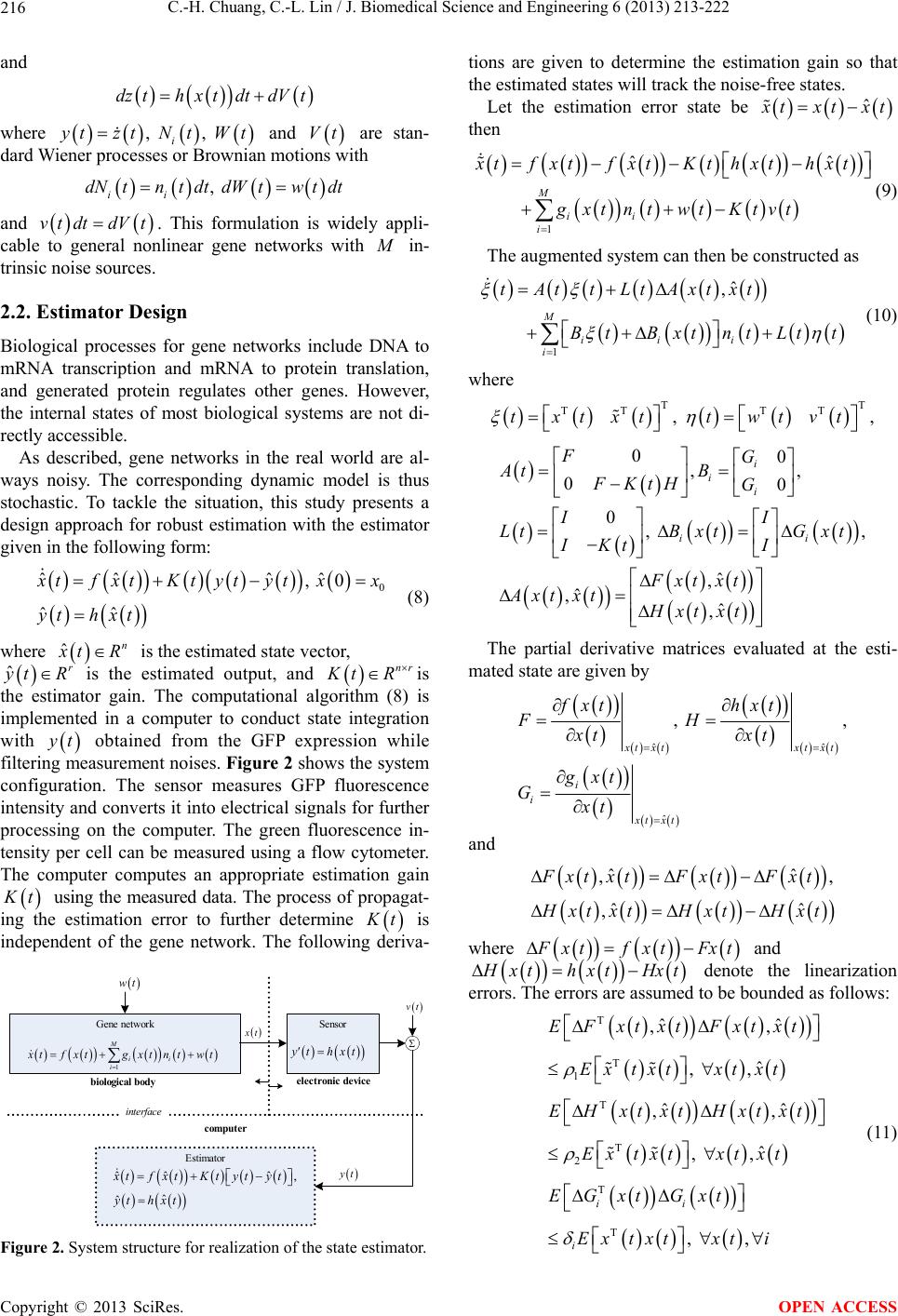 C.-H. Chuang, C.-L. Lin / J. Biomedical Science and Engineering 6 (2013) 213-222 216 and dz thx tdtdVt where , tzt , i Nt Wt and are stan- dard Wiener processes or Brownian motions with Vt , ii dNtntdtdWtw tdt and . This formulation is widely appli- cable to general nonlinear gene networks with v tdtdVt in- trinsic noise sources. 2.2. Estimator Design Biological processes for gene networks include DNA to mRNA transcription and mRNA to protein translation, and generated protein regulates other genes. However, the internal states of most biological systems are not di- rectly accessible. As described, gene networks in the real world are al- ways noisy. The corresponding dynamic model is thus stochastic. To tackle the situation, this study presents a design approach for robust estimation with the estimator given in the following form: 0 ˆˆˆˆ , 0 ˆˆ tf xtKtytytxx yt hxt (8) where ˆn tR r R is the estimated state vector, ˆ yt is the estimated output, and nr tR is the estimator gain. The computational algorithm (8) is implemented in a computer to conduct state integration with t obtained from the GFP expression while filtering measurement noises. Figure 2 shows the system configuration. The sensor measures GFP fluorescence intensity and conv erts it into electrical signals for further processing on the computer. The green fluorescence in- tensity per cell can be measured using a flow cytometer. The computer computes an appropriate estimation gain t using the measured data. The process of propagat- ing the estimation error to further determine t is independent of the gene network. The following deriva- Estimator G ene networkSensor 1 M ii i tfxtgxtntwt t yt hxt ˆˆ ˆ, ˆˆ tfxtKtytyt yt hxt t vt interface compute r biolog ical b o dy electronic device wt Figure 2. System structure for realization of the state estimator. tions are given to determine the estimation gain so that the estimated states will track the noise-free states. Let the estimation error state be ˆ txtxt then 1 ˆˆ M ii i tfxt fxtKthxthxt gxtntwtKtvt (9) The augmented system can then be constructed as 1 ˆ , M iii i tAttLtAxtxt BtBxt ntLtt (10) where TT TT TT , ,txtxttwtvt 00 ,, 00 0, , ˆ , ˆ ,ˆ , i ii ii FG At B FKtH G II LtB xtG xt IKt I Fxt xt Axt xtHxt xt The partial derivative matrices evaluated at the esti- mated state are given by ˆˆ ˆ , , txt xtxt i i xtxt fxthxt FH xt xt gxt Gxt and ˆˆ ,, ˆˆ , xt xtFxtFxt xtxtH xtHxt where xtf xtFxt and xthxt Hxt denote the linearization errors. The errors are assumed to be bounded as follows: T T 1 T T 2 T T ˆˆ ,, ˆ , , ˆˆ ,, ˆ , , , , ii i EFxtxtFxtxt Extxtxt xt EHxtxtHxtxt Extxtxt xt EGxt Gxt Ex txtxti (11) Copyright © 2013 SciRes. OPEN ACCESS 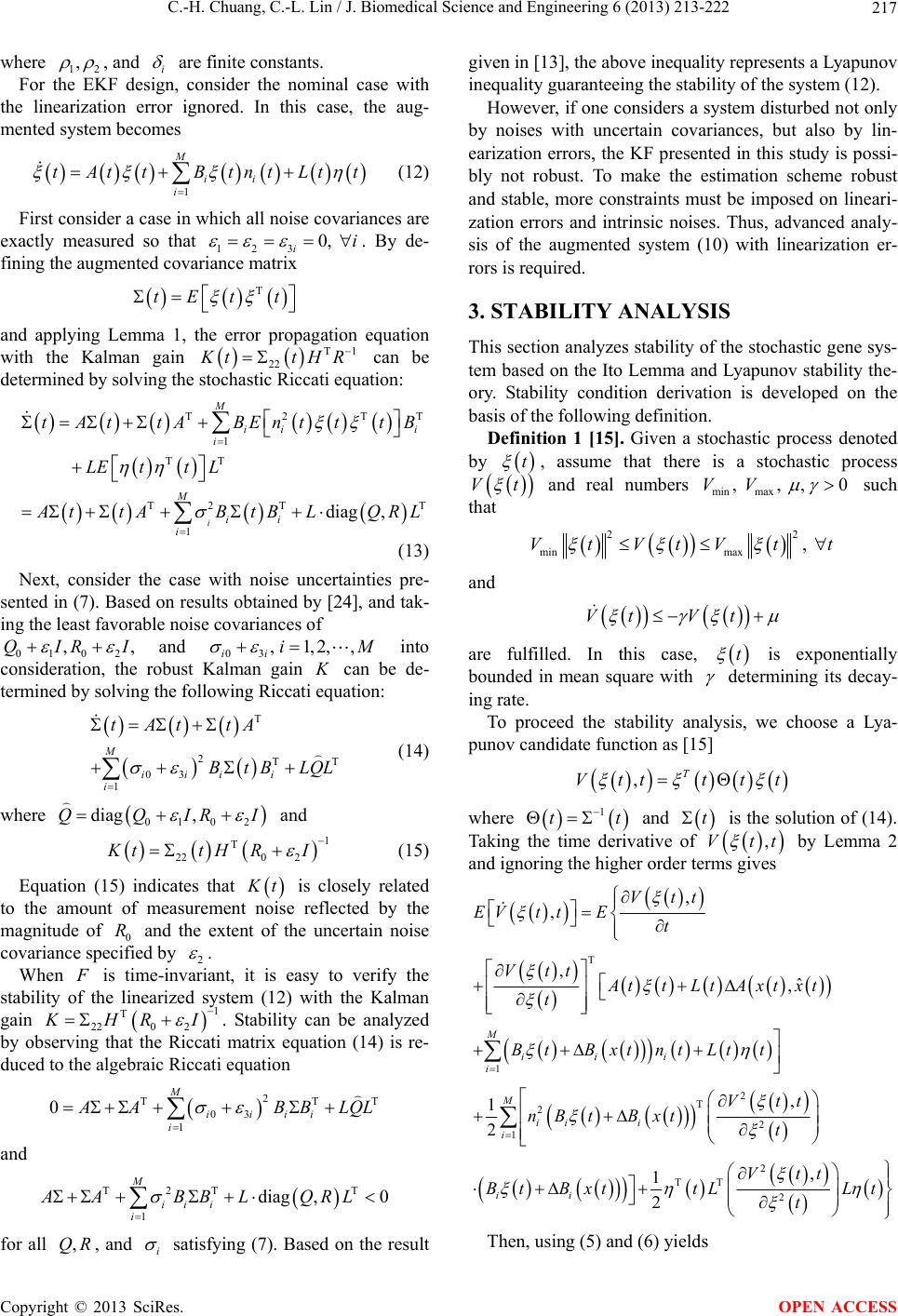 C.-H. Chuang, C.-L. Lin / J. Biomedical Science and Engineering 6 (2013) 213-222 217 where 12 , , and i are finite constants. For the EKF design, consider the nominal case with the linearization error ignored. In this case, the aug- mented system becomes 1 M ii i tAtt BtntLtt (12) First consider a case in which all noise covariances are exactly measured so that 123 0, ii . By de- fining the augmented covariance matrix T tEtt and applying Lemma 1, the error propagation equation with the Kalman gain1 22 T ttH R can be determined by solving the stochastic Riccati equation: T T T2T 1 TT T2 T 1diag , i M ii i i M ii i tAttABEntt tB LEttL ttABtBL QR L , I (13) Next, consider the case with noise uncertainties pre- sented in (7). Based on results obtained by [24], and tak- ing the least favorable noise covariances of 0102 ,QIR and 03 , 1,2,, ii iM into consideration, the robust Kalman gain can be de- termined by solving the following Riccati equation: T T 2T 03 1 M iii i i tAttA BtB LQL (14) where 0102 diag ,QQIRI and 1 220 2 T ttHRI (15) Equation (15) indicates that t is closely related to the amount of measurement noise reflected by the magnitude of 0 and the extent of the uncertain noise covariance specified by R 2 . When is time-invariant, it is easy to verify the stability of the linearized system (12) with the Kalman gain 0 2 1 T 22 HR I . Stability can be analyzed by observing that the Riccati matrix equation (14) is re- duced to the algebraic Riccati equation 2 TT 03 1 0M iiii i T ABB LQL and T2T T 1 diag ,0 M ii i i AABBL QRL for all , and ,QR i satisfying (7). Based on the result given in [13], the above inequality represen ts a Lyapunov inequality guaranteein g the stability of the system (12). However, if one considers a system disturbed not only by noises with uncertain covariances, but also by lin- earization errors, the KF presented in this study is possi- bly not robust. To make the estimation scheme robust and stable, more constraints must be imposed on lineari- zation errors and intrinsic noises. Thus, advanced analy- sis of the augmented system (10) with linearization er- rors is required. 3. STABILITY ANALYSIS This section analyzes stability of the stochastic gene sys- tem based on the Ito Lemma and Lyapunov stability the- ory. Stability condition derivation is developed on the basis of the following definition. Definition 1 [15]. Given a stochastic process denoted by t , assume that there is a stochastic process t V and real numbers min max , , ,0VV such that 22 minmax , VtVtVt t and Vt Vt are fulfilled. In this case, t is exponentially bounded in mean square with determining its decay- ing rate. To proceed the stability analysis, we choose a Lya- punov candidate function as [15] ,T Vttttt where 1 t t and is the solution of (14). Taking the time derivative of by Lemma 2 and ignoring the higher order terms gives t ,Vtt T 1 2 T 2 2 1 2 TT 2 , , ,ˆ , , 1 2 , 1 2 M iii i M ii i i ii Vtt EVt tEt Vtt AttLtAxt xt t BtBxtntLt t Vtt nB tBxtt Vtt tBxttLLt t Then, using ( 5) and (6) yields Copyright © 2013 SciRes. OPEN ACCESS 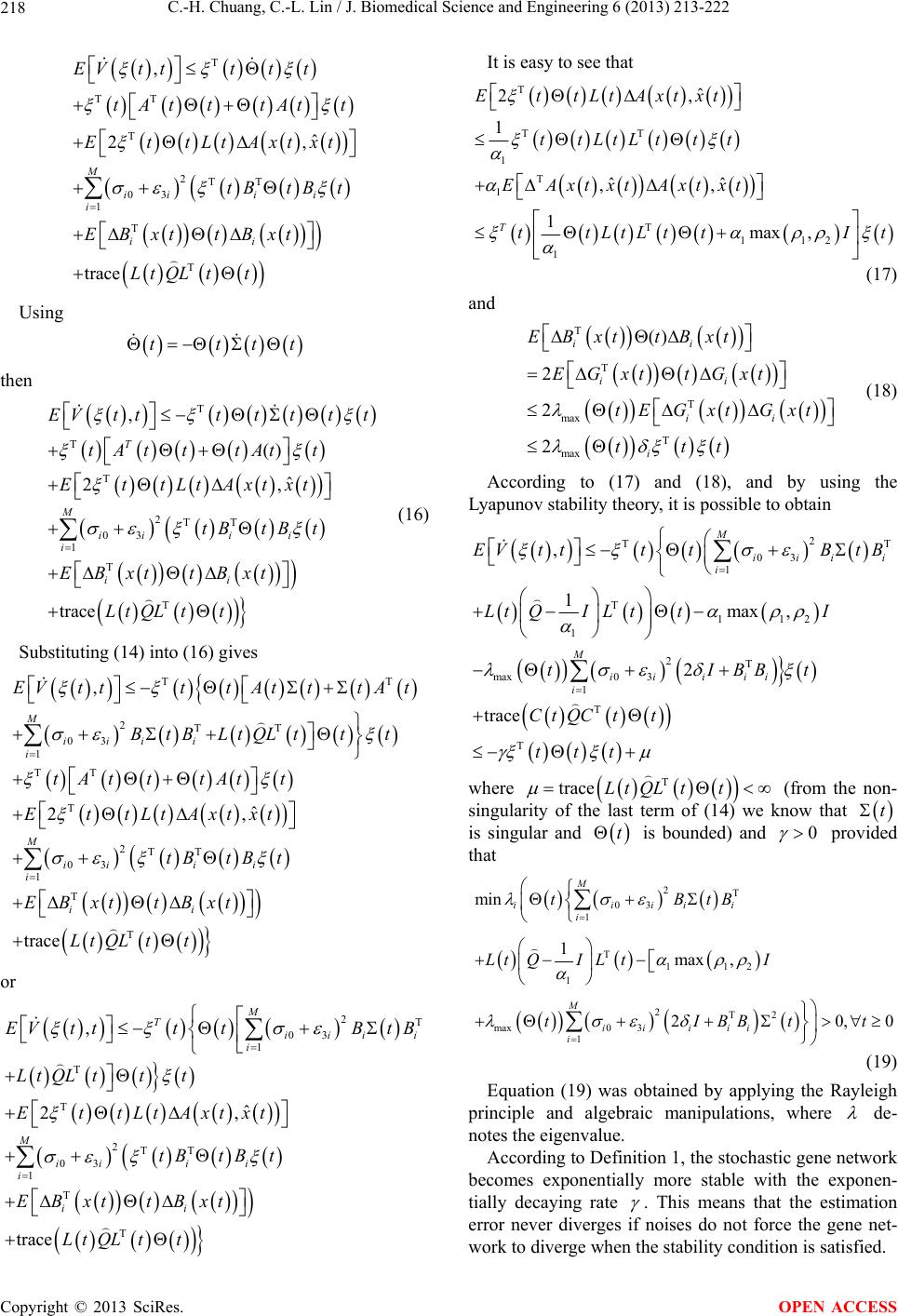 C.-H. Chuang, C.-L. Lin / J. Biomedical Science and Engineering 6 (2013) 213-222 218 T TT T 2TT 03 1 T T , ˆ 2, trace M iii i i ii EVt tttt tAtttAtt EttLtAxt xt tBtBt EBxt tBxt LtQL tt Using ttt t then T T T 2TT 03 1 T T , () ˆ 2, trace T M iii i i ii EVtt ttttt tAtttAtt EttLtAxt xt tBtBt EBxt tBxt LtQL tt i (16) Substituting (14) in to (16) gives TT 2TT 03 1 TT T 2TT 03 1 T T , ˆ 2, trace M iii i i M iii i i ii EVt tttAtttAt BtBLtQLttt tAtttAtt EttLtAxt xt tBtB t EBxt tBxt LtQL tt or 2T 03 1 T T 2TT 03 1 T T , ˆ 2, trace M Tiii i M iii i i ii EVt tttBtB LtQL ttt EttLtAxt xt tBtBt EBxt tBxt LtQL tt It is easy to see that T TT 1 T 1 T112 1 ˆ 2, 1 ˆˆ ,, 1max , T EttLtAxt xt ttLtLttt EAxt xtAxt xt ttLtLtt I t (17) and T T T max T max () 2 2 2 ii ii ii i EBxttB xt EGxttG xt tE GxtGxt ttt (18) According to (17) and (18), and by using the Lyapunov stability theory, it is possible to obtain 2 TT 03 1 T112 1 2T max0 3 1 T T , 1max , 2 trace M iii i M ii iii i EVt tttBtB LtQI LttI tIBBt CtQC tt ttt i where T trace LtQL tt (from the non- singularity of the last term of (14) we know that t is singular and t is bounded) and 0 provided that 2T 03 1 T112 1 2T2 max0 3 1 min 1max , 20 M iiiii i M ii iii i tBtB LtQI LtI tIBBt ,0t (19) Equation (19) was obtained by applying the Rayleigh principle and algebraic manipulations, where de- notes the eigenvalue. According to Definition 1, the stochastic gene network becomes exponentially more stable with the exponen- tially decaying rate . This means that the estimation error never diverges if noises do not force the gene net- work to diverge when the stability condition is satisfied. Copyright © 2013 SciRes. OPEN ACCESS 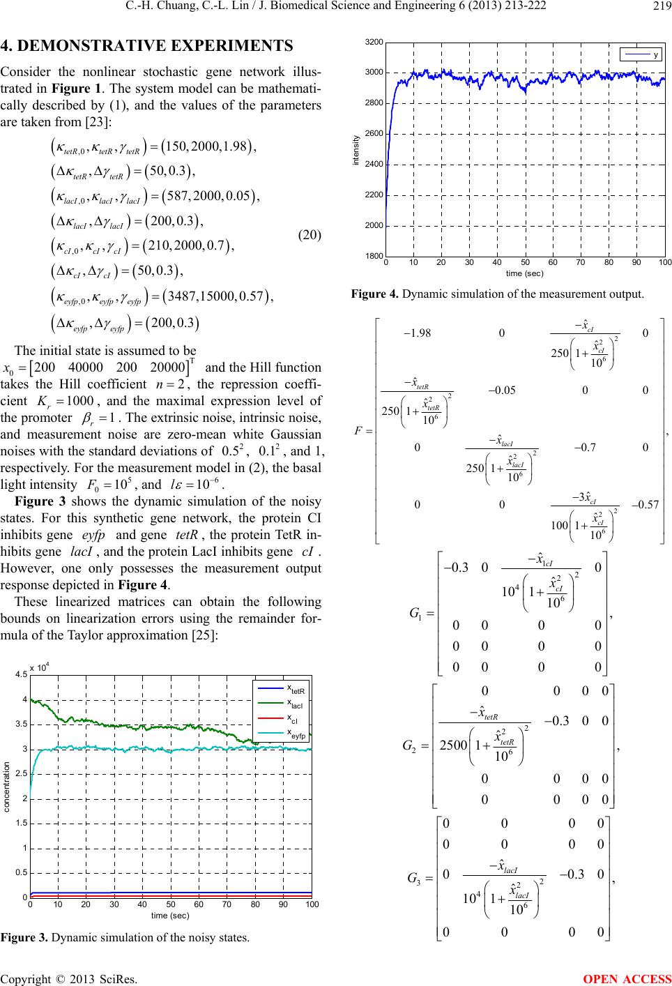 C.-H. Chuang, C.-L. Lin / J. Biomedical Science and Engineering 6 (2013) 213-222 219 4. DEMONSTRATIVE EXPERIMENTS Consider the nonlinear stochastic gene network illus- trated in Figure 1. The system model can be mathemati- cally described by (1), and the values of the parameters are taken from [23]: ,0 ,0 ,0 ,0 ,,150,2000,1.98 , ,50,0.3, ,,587,2000,0.05, ,200,0.3, ,,210,2000,0.7 , ,50,0.3, ,,3487,15000,0.57 , , tetRtetR tetR tetR tetR lacIlacIlacI lacI lacI cIcIcI cI cI eyfpeyfp eyfp eyfp 200,0.3 eyfp (20) The initial state is assumed to be and the Hill function takes the Hill coefficient T 0200 40000 200 20000x2n , the repression coeffi- cient , and the maximal expression level of the promoter 1000 r K1 r 5 010F10l . The extrinsic noise, intrinsic noise, and measurement noise are zero-mean white Gaussian noises with the standard deviations of , , and 1, respectively. For the measurement model in (2), th e basal light intensity , and . 2 0.5 6 2 0.1 Figure 3 shows the dynamic simulation of the noisy states. For this synthetic gene network, the protein CI inhibits gene and gene te, the protein TetR in- hibits gene , and the protein LacI inhibits gene . However, one only possesses the measurement output response depicted in Figure 4. eyfp lacI tR cI These linearized matrices can obtain the following bounds on linearization errors using the remainder for- mula of the Taylor approximation [25]: 010 2030 40 5060 708090 100 0 0.5 1 1.5 2 2.5 3 3.5 4 4.5 x 10⁴ time (sec) c o ncen t ration x tetR x lacI x cI x eyfp Figure 3. Dynamic simulation of the noisy states. 010 2030 4050 60 70 8090100 1800 2000 2200 2400 2600 2800 3000 3200 time (sec) intensity y Figure 4. Dynamic simulation of the measurement output. 2 2 6 2 2 6 2 2 6 2 2 6 ˆ 1.98 00 ˆ 250 110 ˆ0.050 0 ˆ 250 110 , ˆ 00.7 ˆ 250 110 ˆ 3 0 00.57 ˆ 100 110 cI cI tetR tetR lacI lacI cI cI x x x x Fx x x x 0 12 2 46 1 ˆ 0.3 00 ˆ 10110 , 0000 0000 0000 cI cI x x G 2 2 26 000 ˆ0.3 0 0 ˆ, 2500 110 000 000 tetR tetR x x G 0 0 0 2 32 46 00 0 00 0 ˆ 00 , ˆ 10110 00 0 lacI lacI x Gx 0 0 .30 0 Copyright © 2013 SciRes. OPEN ACCESS 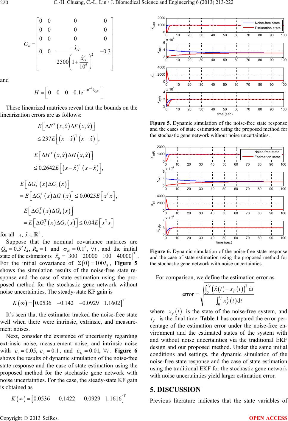 C.-H. Chuang, C.-L. Lin / J. Biomedical Science and Engineering 6 (2013) 213-222 220 4 2 2 6 00 00 00 00 00 00 ˆ 00 0.3 ˆ 2500 110 cI cI Gx x and 6ˆ 10 0000.1eeyfp x H These linearized matrices reveal that the bounds on the linearization errors are as follows: T T ˆˆ ,, ˆˆ 237 , EFxxFxx Exx xx T T ˆˆ ,, ˆˆ 0.2642 , EHxxHxx Exx xx T 33 TT 11 0.0025 , EGxGx EGxGx Exx T 44 TT 22 0.04 EGxGx EGxGx Exx 4 for all . ˆ , xx Suppose that the nominal covariance matrices are and 2 040 0.5, 1QIR 2 00.1, ii 300 20000 01 , and the initial state of the estimator is . For the initial covariance of 8 T 0 ˆ10040000x00 , Figure 5 shows the simulation results of the noise-free state re- sponse and the case of state estimation using the pro- posed method for the stochastic gene network without noise uncertainties. The steady-state KF gain is T 0.05360.1420.0929 1.1602K It’s seen that the estimator tracked the noise-free state well when there were intrinsic, extrinsic, and measure- ment noises. Next, consider the existence of uncertainty regarding extrinsic noise, measurement noise, and intrinsic noise with 12 0.05, 0.1 , and 30.01, ii . Figure 6 shows the results of dynamic simulation of the noise-free state response and the case of state estimation using the proposed method for the stochastic gene network with noise uncertainties. For the case, the steady-state KF gain is obtained as T 0.05360.14220.0929 1.1616K 010 2030 4050 60 708090 100 0 1000 2000 x tetR Nois e-f ree s tate Esti m ation state 010 2030 4050 60 7080 90 6x 10 4 100 2 4 x lacI 4000 2000 010 2030 4050 60 708090 100 0 x cI 010 2030 4050 60 7080 90 4x 10 4 3 2100 x ey fp time (sec) Figure 5. Dynamic simulation of the noise-free state response and the cases of state estimation using the proposed method for the stochastic gene network without noise uncertainties. 01020 30 4050 60 70 80 90100 0 1000 2000 x tetR Nois e-f ree stat e Est i m ati on state 01020 30 4050 60 70 80 90 6x 10 4 100 2 4 x lacI 4000 2000 01020 30 4050 60 70 80 90100 0 x cI 01020 30 4050 60 70 80 90 4x 10 4 3 2100 x ey fp time (sec) Figure 6. Dynamic simulation of the noise-free state response and the case of state estimation using the proposed method for r as the stochastic gene network with noise uncertainties. For comparison, we define the estimation erro 2 0ˆd error f t f 2 0d f t f txt t xtt where f t is the state of the noise-freesystem, and t is thl time. Table 1 has compared the error per- vi Previous literature indicates that the state variables of e fina of thcentagee estimation error under the noise-free en- ronment and the estimated states of the system with and without noise uncertainties via the traditional EKF design and our proposed method. Under the same initial conditions and settings, the dynamic simulation of the noise-free state response and the case of state estimation using the traditio nal EKF for the stochastic g ene network with noise uncertainties yield larger estimation error. 5. DISCUSSION Copyright © 2013 SciRes. OPEN ACCESS 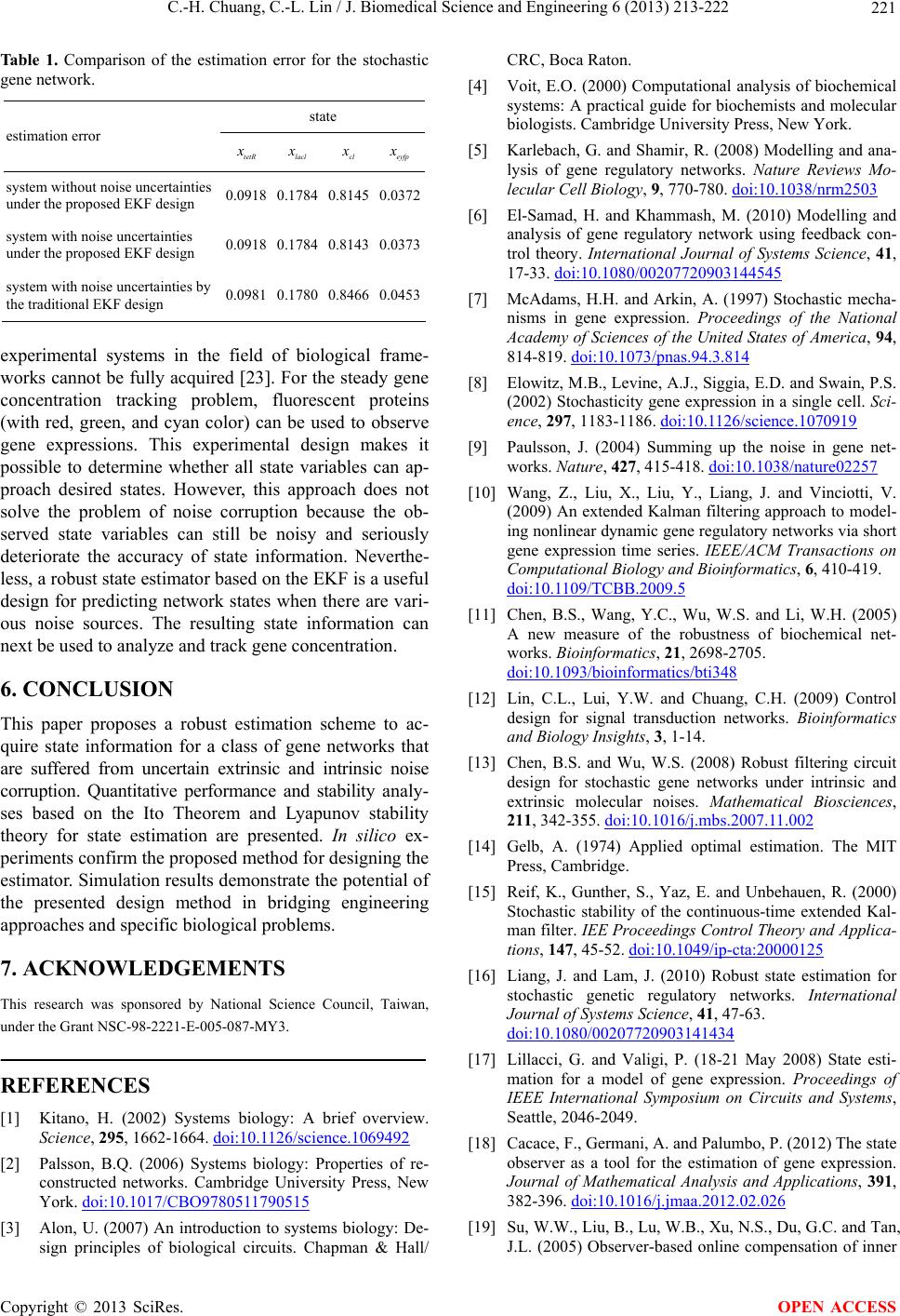 C.-H. Chuang, C.-L. Lin / J. Biomedical Science and Engineering 6 (2013) 213-222 221 Table 1. Comparison of the estimation error for the stochastic gene network. state estimation error tetR lacl cl eyfp system without n under the proposed oise uncertainties EKF design 0.0918 0.1784 0.81450.0372 system with noise uncertainties under the proposed EKF design 0.0918 0.1784 0.81430.0373 system with noise uncertainties by the traditional EKF design 0.0981 0.1780 0.84660.0453 orks cannot be fully acquired [23]. For the steady ge This paper proposes a robust estimation scheme to ac- or a class of gene networks that This research was sponsored by National Science Council, Taiwan, -1664. doi:10.1126/science.1069492 experimental systems in the field of biological frame- wne concentration tracking problem, fluorescent proteins (with red, green, and cyan color) can be used to observe gene expressions. This experimental design makes it possible to determine whether all state variables can ap- proach desired states. However, this approach does not solve the problem of noise corruption because the ob- served state variables can still be noisy and seriously deteriorate the accuracy of state information. Neverthe- less, a robust state estimator based on the EKF is a useful design for predicting network states when there are vari- ous noise sources. The resulting state information can next be used to analyze and track gene concentration. 6. CONCLUSION quire state information f are suffered from uncertain extrinsic and intrinsic noise corruption. Quantitative performance and stability analy- ses based on the Ito Theorem and Lyapunov stability theory for state estimation are presented. In silico ex- periments confirm the propo sed method for designing th e estimator. Simulation results demonstrate the poten tial of the presented design method in bridging engineering approaches and specific biological pr oblems. 7. ACKNOWLEDGEMENTS under the Grant NSC-98-2221-E-005-087-MY3. REFERENCES [1] Kitano, H. (2002) Systems biology: A brief overview. Science, 295, 1662 [2] Palsson, B.Q. (2006) Systems biology: Properties of re- constructed networks. Cambridge University Press, New York. doi:10.1017/CBO9780511790515 [3] Alon, U. (2007) An introduction to systems biology: De- sign principles of biological circuits. Chapman & Hall/ CRC, Boca Raton. [4] Voit, E.O. (2000) Computational analysis of biochemical systems: A practical guide for biochemists and molecular biologists. Cambridge University Press, New York. 03 [5] Karlebach, G. and Shamir, R. (2008) Modelling and ana- lysis of gene regulatory networks. Nature Reviews Mo- lecular Cell Biology, 9, 770-780. doi:10.1038/nrm25 1, [6] El-Samad, H. and Khammash, M. (2010) Modelling and analysis of gene regulatory network using feedback con- trol theory. International Journal of Systems Science, 4 17-33. doi:10.1080/00207720903144545 [7] McAdams, H.H. and Arkin, A. (1997) Stochastic mecha- nisms in gene expression. Proceedings of the National Academy of Sciences of the United States of America, 94, 814-819. doi:10.1073/pnas.94.3.814 [8] Elowitz, M.B., Levine, A.J., Siggia, E.D. and Swain, P.S. (2002) Stochasticity gene expression in a single cell. Sci- ence, 297, 1183-1186. doi:10.1126/science.1070919 [9] Paulsson, J. (2004) Summing up the noise in gene net- works. Nature, 427, 415-418. doi:10.1038/nature02257 [10] Wang, Z., Liu, X., Liu, Y., Liang, J. and Vinciotti, V. rt (2009) An extended Kalman filtering approach to model- ing nonlinear dynamic gene regulatory networks via sho gene expression time series. IEEE/ACM Transactions on Computational Biology and Bioinformatics, 6, 410-419. doi:10.1109/TCBB.2009.5 [11] Chen, B.S., Wang, Y.C., Wu, W.S. and Li, W.H. (2005) A new measure of the robustness of biochemical net- works. Bioinformatics, 21, 2698-2705. doi:10.1093/bioinformatics/bti348 [12] Lin, C.L., Lui, Y.W. and Chuang, C.H. (2009) Control design for signal transduction network and Biology Insights, 3, 1-14. s. Bioinformatics athematical Biosciences, [13] Chen, B.S. and Wu, W.S. (2008) Robust filtering circuit design for stochastic gene networks under intrinsic and extrinsic molecular noises. M 211, 342-355. doi:10.1016/j.mbs.2007.11.002 [14] Gelb, A. (1974) Applied optimal estimation. The MIT Press, Cambridge. [15] Reif, K., Gunther, S., Yaz, E. and Unbehauen, R. (2000) ceedings Control Theory and Applica- Stochastic stability of the continuous-time extended Kal- man filter. IEE Pro tions, 147, 45-52. doi:10.1049/ip-cta:20000125 [16] Liang, J. and Lam, J. (2010) Robust state estimation for stochastic genetic regulatory networks. International Journal of Systems Science, 41, 47-63. doi:10.1080/00207720903141434 [17] Lillacci, G. and Valigi, P. (18-21 May 2008) State esti- mation for a model of gene expressio IEEE International Symposium onn. Proceedings of Circuits and Systems, tical Analysis and Applications, 391, Seattle, 2046-2049. [18] Cacace, F., Germani, A. and Palumbo, P. (2012) The state observer as a tool for the estimation of gene expression. Journal of Mathema 382-396. doi:10.1016/j.jmaa.2012.02.026 [19] Su, W.W., Liu, B., Lu, W.B., Xu, N.S., Du, G.C. and Ta n, J.L. (2005) Observer-based online compensation of inner Copyright © 2013 SciRes. OPEN ACCESS  C.-H. Chuang, C.-L. Lin / J. Biomedical Science and Engineering 6 (2013) 213-222 Copyright © 2013 SciRes. 222 FP-expre OPEN ACCESS filter effect in monitoring fluorescence of Gssing plant cell cult ures. Biotechnology and Bioengineering, 91, 213-226. doi:10.1002/bit.20510 [20] Chuang, C.H. and Lin, C.L. (2010) On robust state esti- mation of gene networks. Biomedical Engineering and Computational Biology, 2, 23-36. nd Control, Shanghai, bust synthetic biology to satisfy design [21] Choukroun, D. (16-18 December 2009) Ito stochastic modeling for attitude quaternion filtering. Proceedings of IEEE Conference on Decision a 733-738. [22] Gardiner, C.W. (1980) Handbook of stochastic methods of differential equations. Sijthoff and Noordhoff, Alphen aan den Rijn. [23] Chen, B.S. and Wu, C.H. (2009) A systematic design method for ro specifications. BMC Systems Biology, 3, 1-18. doi:10.1186/1752-0509-3-66 [24] Poor, V. and Looze, D.P. (1981) Minimax sta tion for linear stochastic systems withte estima- noise uncertainty. IEEE Transactions on Automatic Control, 26, 902-906. doi:10.1109/TAC.1981.1102756 [25] Bartle, S. (2000) Introduction to real analysis. 3rd Editio John Wiley & Sons, New York. n,
|