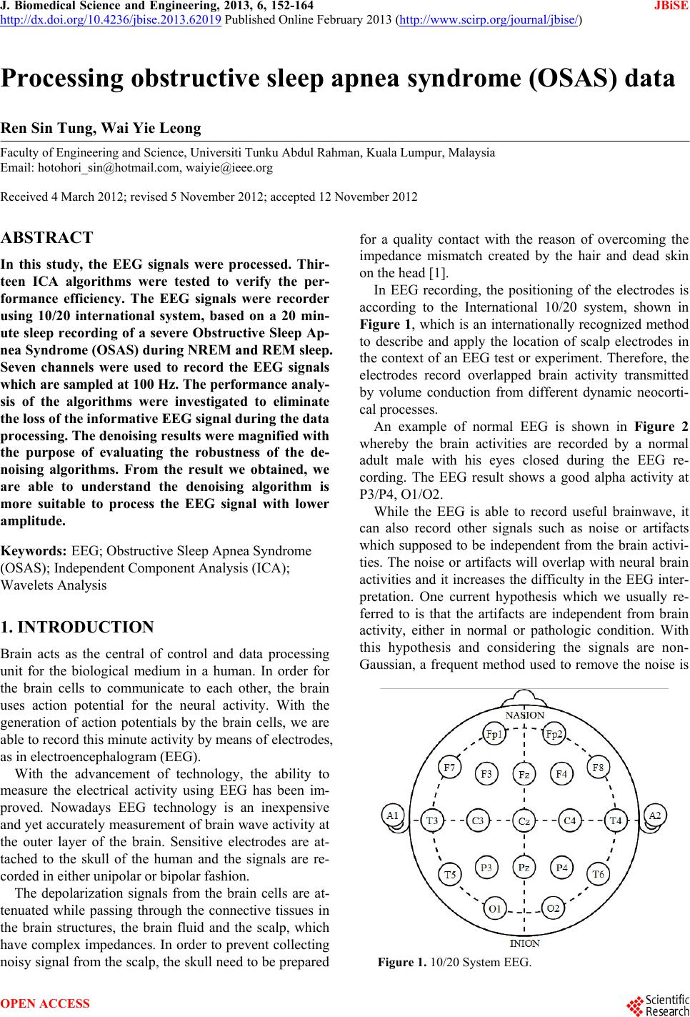
 J. Biomedical Science and Engineering, 2013, 6, 152-164 JBiSE http://dx.doi.org/10.4236/jbise.2013.62019 Published Online February 2013 (http://www.scirp.org/journal/jbise/) Processing obstructive sleep apnea syndrome (OSAS) data Ren Sin Tung, Wai Yie Leong Faculty of Engineering and Science, Universiti Tunku Abdul Rahman, Kuala Lumpur, Malaysia Email: hotohori_sin@hotmail.com, waiyie@ieee.org Received 4 March 2012; revised 5 November 2012; accepted 12 November 2012 ABSTRACT In this study, the EEG signals were processed. Thir- teen ICA algorithms were tested to verify the per- formance efficiency. The EEG signals were recorder using 10/20 international system, based on a 20 min- ute sleep recording of a severe Obstructive Sleep Ap- nea Syndrome (OSAS) during NREM and REM sleep. Seven channels were used to record the EEG signals which are sampled at 100 Hz. The performance analy- sis of the algorithms were investigated to eliminate the loss of the informative EEG signal during the data processing. The denoising results were magnified with the purpose of evaluating the robust ness of the de- noising algorithms. From the result we obtained, we are able to understand the denoising algorithm is more suitable to process the EEG signal with lower amplitude. Keywords: E EG; Obstructive Sleep Apnea Syndrome (OSAS); Independent Component Analysis (ICA); Wavelets Analysis 1. INTRODUCTION Brain acts as the central of control and data processing unit for the biological medium in a human. In order for the brain cells to communicate to each other, the brain uses action potential for the neural activity. With the generation of action potentials by the brain cells, we are able to record this minute activity by means of electrodes, as in electroencephalogram (EEG). With the advancement of technology, the ability to measure the electrical activity using EEG has been im- proved. Nowadays EEG technology is an inexpensive and yet accurately measurement of brain wave activity at the outer layer of the brain. Sensitive electrodes are at- tached to the skull of the human and the signals are re- corded in either unipolar or bipolar fashion. The depolarization signals from the brain cells are at- tenuated while passing through the connective tissues in the brain structures, the brain fluid and the scalp, which have complex impedances. In order to prevent collecting noisy signal from the scalp, the skull need to be prepared for a quality contact with the reason of overcoming the impedance mismatch created by the hair and dead skin on the head [1] . In EEG recording, the positioning of the electrodes is according to the International 10/20 system, shown in Figure 1, which is an internationally recognized method to describe and apply the location of scalp electrodes in the context of an EEG test or experiment. Therefore, the electrodes record overlapped brain activity transmitted by volume conduction from different dynamic neocorti- cal processes. An example of normal EEG is shown in Figure 2 whereby the brain activities are recorded by a normal adult male with his eyes closed during the EEG re- cording. The EEG result shows a good alpha activity at P3/P4, O1/O2. While the EEG is able to record useful brainwave, it can also record other signals such as noise or artifacts which supposed to be independent from the brain activi- ties. The noise or artifacts will overlap with neural brain activities and it increases the difficulty in the EEG inter- pretation. One current hypothesis which we usually re- ferred to is that the artifacts are independent from brain activity, either in normal or pathologic condition. With this hypothesis and considering the signals are non- Gaussian, a frequent method used to remove the noise is Figure 1. 10/20 System EEG. OPEN ACCESS 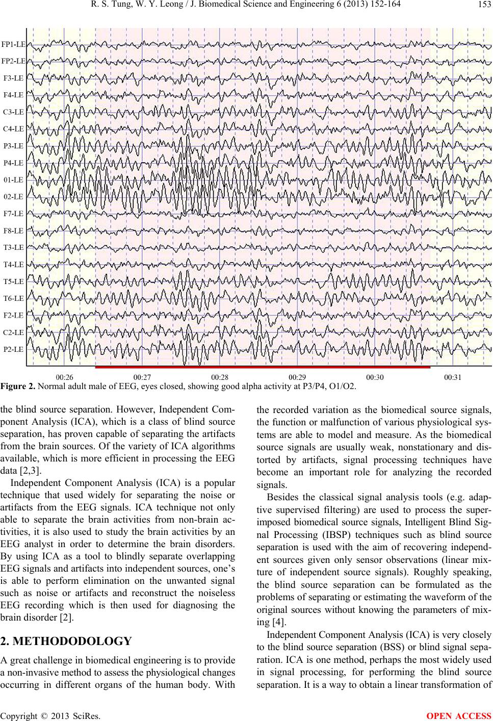 R. S. Tung, W. Y. Leong / J. Biomedical Science and Engineering 6 (2013) 152-164 153 Figure 2. Normal adult male of EEG, eyes closed, showing good alpha activity at P3/P4, O1/O2. the blind source separation. However, Independent Com- ponent Analysis (ICA), which is a class of blind source separation, has proven capable of separating the artifacts from the brain sources. Of the variety of ICA algorithms available, which is more efficient in processing the EEG data [2,3]. Independent Component Analysis (ICA) is a popular technique that used widely for separating the noise or artifacts from the EEG signals. ICA technique not only able to separate the brain activities from non-brain ac- tivities, it is also used to study the brain activities by an EEG analyst in order to determine the brain disorders. By using ICA as a tool to blindly separate overlapping EEG signals and artifacts into independ en t sources, on e’s is able to perform elimination on the unwanted signal such as noise or artifacts and reconstruct the noiseless EEG recording which is then used for diagnosing the brain disorder [2]. 2. METHODODOLOGY A great challenge in biomedical engineering is to provide a non-invasive method to assess the physiological chan ges occurring in different organs of the human body. With the recorded variation as the biomedical source signals, the function or malfunction of various physiological sys- tems are able to model and measure. As the biomedical source signals are usually weak, nonstationary and dis- torted by artifacts, signal processing techniques have become an important role for analyzing the recorded signals. Besides the classical signal analysis tools (e.g. adap- tive supervised filtering) are used to process the super- imposed biomedical source signals, Intelligent Blind Sig- nal Processing (IBSP) techniques such as blind source separation is used with the aim of recovering independ- ent sources given only sensor observations (linear mix- ture of independent source signals). Roughly speaking, the blind source separation can be formulated as the problems of separating or estimating the waveform of the original sources without knowing the parameters of mix- ing [4]. Independent Component Analysis (ICA) is very clo se ly to the blind source separation (BSS) or blind signal sepa- ration. ICA is one method, perhaps the most widely used in signal processing, for performing the blind source separation. It is a way to obtain a linear transformation of Copyright © 2013 SciRes. OPEN ACCESS  R. S. Tung, W. Y. Leong / J. Biomedical Science and Engineering 6 (2013) 152-164 154 the measured signals such that the resulting source sig- nals are statistically independent from each other. To generally define ICA, statistical “latent variables” model is used for the definition. Assuming the observed linear mixtures 1,, n x of n independent components: 112 2,for all. jj jjnn as asasj (1) By leaving the time index t in the ICA model, each mixture xj as well as each independent component sk is assumed to be a random variable instead of a proper time signal. The observed values xj(t) are then a sample of this random variable. Without the loss of generality, both th e mixture variables and the independent components are assumed to be zero mean . For the convenient purpose, vector-matrix notation is used instead of the sum like in the Equation (1). The random vector of x is denoted by the mixtures 1,, n x and the random vector of s is denoted by the elements 1,, n s. Let us then denote A matrix with the elements of aij whereby the bold lower case letter indicates vector and bold upper case letter denote matrices. By using the vector-matrix notation, the above mixing model is writ- ten as xAs (2) The statistical model in Equation (2) is known as in- dependent component analysis or ICA model. The ICA model is a generative model whereby it describes how the observed data are generated by a process of mixing the components si. In this ICA model, the independents are latent variables, meaning they cannot be observed and the mixing matrix is assumed to be unknown. Ran- dom vector x is observable and this is done under general assumptions. For a random noisy vector x(k), the mixing ICA model can be represented as: kkvxHs k (3) where H is an (m x n) mixing matrix, T 12 ,,, n ksksk sk is a source vector of statistically independent signals (unknown nonsingular mixing matrix), is a T 12 ,,, m vkv kvkvk vector of uncorrelated noise (addictive noise). The purpose of the ICA is to formulate a linear trans- formation W of the dependent sensor signals x that mak e the output as indep endent as possible, yk Wxk WAsk (4) where y is an estimate of the sources (independent com- ponents) and the sources are exactly recovered when the W is the inverse of the A. From Equation (2), there is an ambiguities present in the ICA model. The ambiguity that present in the Equa- tion (2) is that we cannot determine the variances (ener- gies) of the independent components. The reason for the ambiguity is that both s and A being unknow n. Any sca- lar multiplier in one of the sources si could always be cancelled by dividing the corresponding column ai of A by the same scalar. However, this ambiguity is, fortu- nately, insignificant in most application. Besides that, obtaining an exact inverse of the A matrix in most cases is impossible. Thus, the source separation algorithms aim to find a W matrix such as the product of WA in order to permute the diagonal and scalar matrix [4-8]. In the last 20 years, different types of algorithms were proposed and most of the algorithms proposed that the sources are stationary and are based implicitly on high order statistic (HOS) algorithms. With the application of HOS algorithms, Gaussian sources cannot be separated as they do not have higher than two statistic moments while the second order statistic do not have such con- straint. On the other hands, Second Order Statistics (SOS) algorithm uses non stationary structure of the signals (time or frequency structure) for the separation purpose. Temporal, spatial and spatio-temporal decorrelations play important roles in th e EEG signal analysis and these techniques are based on the SOS algorithm. Furthermore, they are the basis for the modern subspace methods of array processing and frequently used to eliminate redun- dancy or to reduce noise. In the spatial decorrelation (pre-whitening) technique, the ICA tasks will usually become easier and well-posed (less ill-conditioned) as the unmixing system is described by an orthogonal ma- trix for real-valued signals and a unitary matrix for com- plex-valued signals and weights. With the same SOS, one’s can compute different whitening transformation for nonstationary sign als. Moreover, the spatio-temporal and time delayed decorrelation can be used to identify the mixing matrix and to perform blind source separation which mainly on coloured source [2]. In contrast to the correlation-based transformation such as principal com- ponent analysis (PCA), ICA not only be able to decorre- late the signals (second order statistic), but it can also reduce higher order statistical dependencies in order to generate signals as independent as possible [3,4,9]. 2.1. SOBI Algorithm One of the well-known second order based technique that used to compute the separating matrix is called Sec- ond Order Blind Identification (SOBI) algorithms. In the SOBI algorithm, the separation of the matrix is achieved in two steps. First step is the whitening the observed signal vector by linear transformation, which is also known as whitening matrix. Second step is applied the Joint Approximate Diagonalization (JAD) on a set of different time-delay correlation matrices of the whitened Copyright © 2013 SciRes. OPEN ACCESS  R. S. Tung, W. Y. Leong / J. Biomedical Science and Engineering 6 (2013) 152-164 155 signal vector. Since the whitening matrix is estimated based on the noisy observed data, it highly suffers from bias if the SNR is relatively low, especially if the noise correlation matrix is unknown. Besides that, the Joint Approximate Diagonalization (JAD) also suffers from highly time correlated noise. In such cases, the correla- tion matrices of the observed signals at nonzero time- delay are still biased by unknown noise correlation ma- trices. In order to overcome the bias of the whitening matrix in white noise cases, robust SOBI algorithm has been developed to overcome the weakness of SOBI al- gorithm [10,11]. 2.2. Robust SOBI Algorithm The robust SOBI (SOBI-RO) algorithm formulates a new correlation matrix as a weighted linear combination of a set of time-delayed correlation matrices of the observed signal vector. The weight linear combination is com- puted in an iterative procedure th at makes the formulated correlation matrix in positive define. The positive define correlation matrix is used for computing the whitening matrix and thereby whitening the observ ed signal vector. In the robust SOBI algorithm, it combines robust whit- ening and time-delayed decorrelation with the purpose of improving the classical SOBI algorithm. By integration the robust whitening instead of simple whitening, the main objective of using robust whitening is to eliminate the influence of whit e noi se [ 11] . Recall the equation introduced in (3), the source sig- nals s are assumed to be mutually uncorrelated and tem- porally correlated (instead of independents) in a second order statistic framework. Computation on this model can be difficult as the presence of noise will influence the correlation between signals. Hence its covariance matrix at lag 0, can be a full T 0 n RE nknk 0 sn s n T c matrix which is unknown and the time-delayed correla- tion matrix will become T n Ri Enknki null. With the above assumption, the correlation matrices of the observation have: TT 0 x RExk xkARAR (5) TT x RiExkxkiARiA R (6) The first step (robust whitening) consists of finding a matrix Q that correlates the signals in x for small time lags. With the helping of ICALAB implementation, which exploits Equation (6) for a single time lag i =1. The matrix Rx(1) is then diagonalized by an eigen-de- composition: diag 22 1N 1 xc RUλλU (7) The whitening matrix Q is then obtained from eigen- vectors matrix Uc and forming a diagonal eigen-valeus matrix diag T 1n QλλUc (8) With the formation of Q matrix, the whitened signal z ki Qxki for different time lags can be calcu- lated. (The default option in ICALAB is 100 time lags). The second step of robust SOBI is the same as the classical SOBI, namely approximate joint diagonaliza- tion of different Rz(i) matrices, computed with the Equa- tion (6). Finally, the separation matrix W is give n by T WAQ (9) where the matrix Q has been computed in the previous whitening or orthogonalization step. Based on the fact that A is an orthogonal matrix and the sources are spa- tially uncorrelated [4,10-12]. 2.3. Wavelet Denoising In a real EEG recording, the recorded signals not only contaminated with ocular or muscular artifacts, it is also contaminated with noises that come from different sources. Currently, in order to remove the noise from the non- stationary signals, Wavelet Denoising (WD) is usually applied for improving the separation result. In WD, the recorded signals are decomposed on wavelet basis. After that, we are able to obtain a representation of the signal that concentrate most of its energy in few wavelet coeffi- cients which having large ab solute values. In the wavelet denoising process, the noise energy distribution does not change, which mean that its energy will not be hold by large value of coefficients. By using large coefficients for denoising, it will lead to an almost noise-free signal. The main problem is the computation of the threshold, which mean responding to where to fix the boundary between the small and large wavelet coefficient? There are a few algorithms have been proposed in the past years and the most well known algorithm is known as Donoho’s universal thresholding. The Donoho’s uni- versal thresholding will compute a threshold level wh e r eb y no Gaussian noise will be left in the denoised signal. However, Donoho’s universal thresholding is able to provide us an almost noise-free signal, but the important drawback of using this thresholding algorithm is the elimination of possibly informative parts of the signal. In the EEG signal analysis, it is important that not to lose potentially useful information during the diagnosis. Moreover, EEG informative signals often have small am- plitude. Therefore, high thresholding algorithm is not ap- propriate for denoising the EEG signal. On the other hands, SURE denoising (Stein Unbiased Risk Estimator) and Minimax methods seem adapted to Copyright © 2013 SciRes. OPEN ACCESS 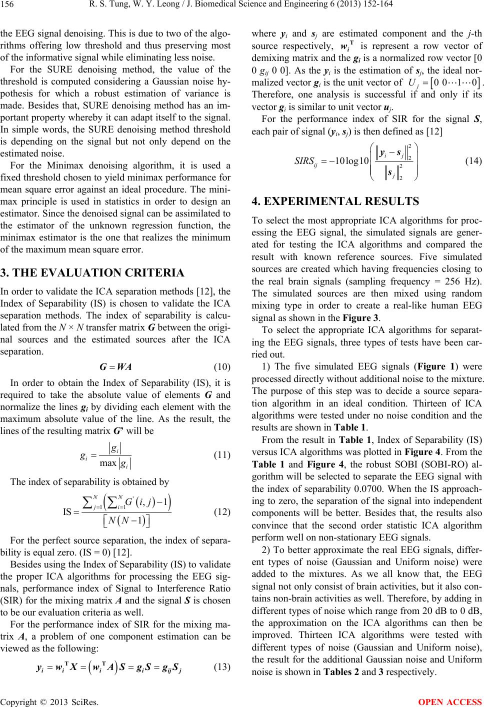 R. S. Tung, W. Y. Leong / J. Biomedical Science and Engineering 6 (2013) 152-164 156 the EEG signal denoising. This is due to two of the algo- rithms offering low threshold and thus preserving most of the informative signal while eliminating less noise. For the SURE denoising method, the value of the threshold is computed considering a Gaussian noise hy- pothesis for which a robust estimation of variance is made. Besides that, SURE denoising method has an im- portant property whereby it can adap t itself to the signal. In simple words, the SURE denoising method threshold is depending on the signal but not only depend on the estimated noise. For the Minimax denoising algorithm, it is used a fixed threshold chosen to yield minimax performance for mean square error against an ideal procedure. The mini- max principle is used in statistics in order to design an estimator. Since the denoised signal can be assimilated to the estimator of the unknown regression function, the minimax estimator is the one that realizes the minimum of the maximum mean square error. 3. THE EVALUATION CRITERIA In order to validate the ICA separation methods [12], the Index of Separability (IS) is chosen to validate the ICA separation methods. The index of separability is calcu- lated from the N × N transfer matrix G between the origi- nal sources and the estimated sources after the ICA separation. GWA (10) In order to obtain the Index of Separability (IS), it is required to take the absolute value of elements G and normalize the lines gi by dividing each element with the maximum absolute value of the line. As the result, the lines of the resulting matrix G’ will be max i ii g g (11) The index of separability is obtained by ' 11 ,1 IS 1 NN ji Gij NN (12) For the perfect source separation, the index of separa- bility is equal zero. (IS = 0) [12]. Besides using the Index of Sep arability (IS) to valid ate the proper ICA algorithms for processing the EEG sig- nals, performance index of Signal to Interference Ratio (SIR) for the mixing matrix A and the signal S is chosen to be our evaluation criteria as well. For the performance index of SIR for the mixing ma- trix A, a problem of one component estimation can be viewed as the following: TT iiii ij where yi and sj are estimated component and the j-th source respectively, is represent a row vector of demixing matrix and the gi is a normalized row vector [0 0 gij 0 0]. As the yi is the estimation of sj, the ideal nor- malized vector gi is the unit vector of T i w 0 010 j U . Therefore, one analysis is successful if and only if its vector gi is similar to unit vector uj. For the performance index of SIR for the signal S, each pair of signal (yi, sj) is then defined as [12] 2 2 2 2 10log10 ij ij j SIRS ys s (14) 4. EXPERIMENTAL RESULTS To select the most appropriate ICA algorithms for proc- essing the EEG signal, the simulated signals are gener- ated for testing the ICA algorithms and compared the result with known reference sources. Five simulated sources are created which having frequencies closing to the real brain signals (sampling frequency = 256 Hz). The simulated sources are then mixed using random mixing type in order to create a real-like human EEG signal as shown in the Figure 3. To select the appropriate ICA algorithms for separat- ing the EEG signals, three types of tests have been car- ried out. 1) The five simulated EEG signals (Figure 1) were processed directly without add itio n al noise to the mixtur e. The purpose of this step was to decide a source separa- tion algorithm in an ideal condition. Thirteen of ICA algorithms were tested under no noise condition and the results are shown in Table 1. From the result in Table 1, Index of Separability (IS) versus ICA algorithms was plotted in Figure 4. From the Table 1 and Figure 4, the robust SOBI (SOBI-RO) al- gorithm will be selected to separate the EEG signal with the index of separability 0.0700. When the IS approach- ing to zero, the separation of the signal into independent components will be better. Besides that, the results also convince that the second order statistic ICA algorithm perform well on non-stationary EEG signals. 2) To better approximate the real EEG signals, differ- ent types of noise (Gaussian and Uniform noise) were added to the mixtures. As we all know that, the EEG signal not only consist of brain activities, but it also co n- tains non-brain activities as well. Therefore, by adding in different types of noise which range from 20 dB to 0 dB, the approximation on the ICA algorithms can then be improved. Thirteen ICA algorithms were tested with different types of noise (Gaussian and Uniform noise), the result for the additional Gaussian noise and Uniform noise is shown in Tables 2 and 3 respectively. j wX wAS S S (13) Copyright © 2013 SciRes. OPEN ACCESS 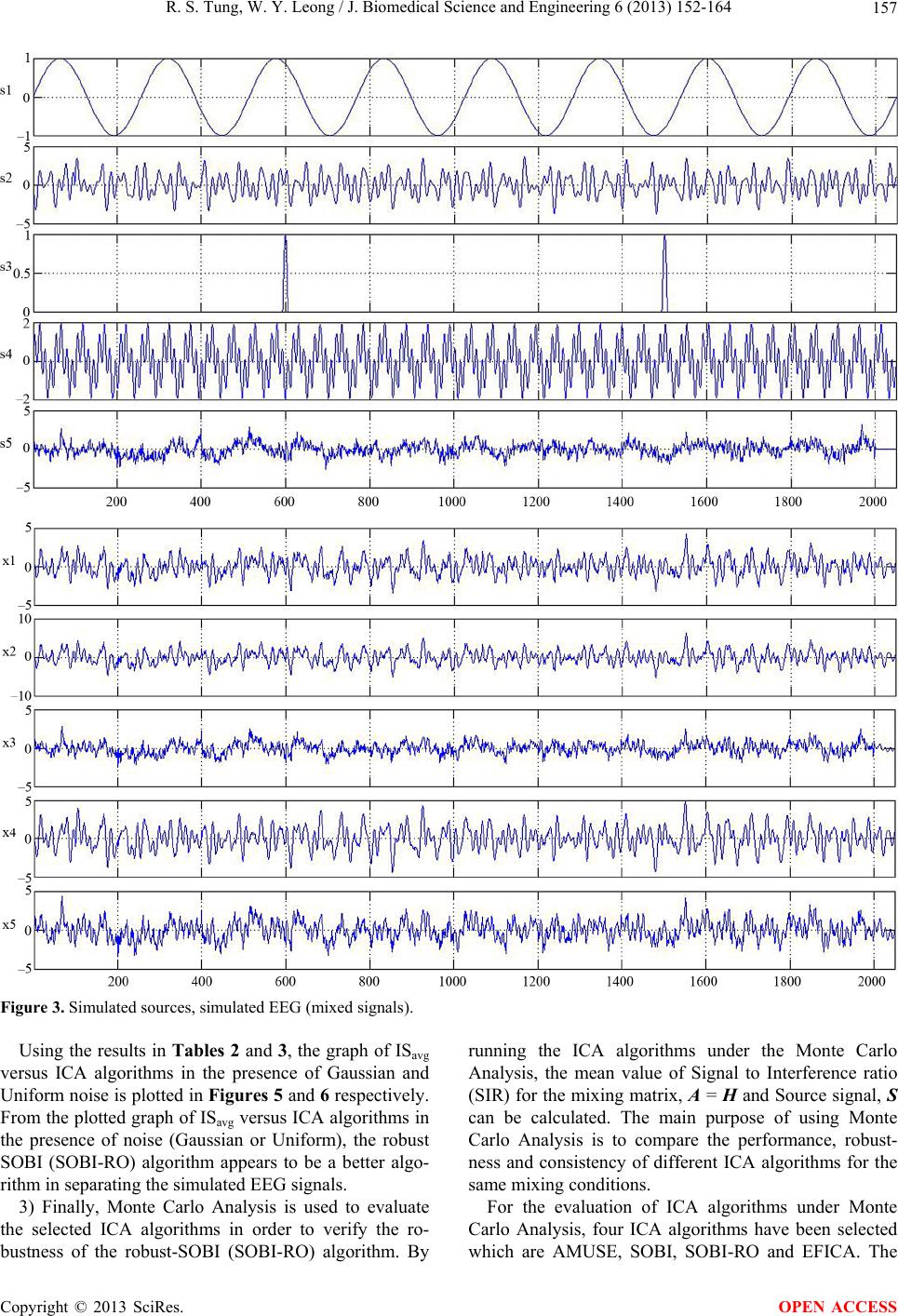 R. S. Tung, W. Y. Leong / J. Biomedical Science and Engineering 6 (2013) 152-164 Copyright © 2013 SciRes. 157 Figure 3. Simulated sources, simulated EEG (mixed signals). Using the results in Tables 2 and 3, the graph of ISavg versus ICA algorithms in the presence of Gaussian and Uniform noise is plotted in Figures 5 and 6 respectively. From the plotted graph of ISavg versus ICA algorithms in the presence of noise (Gaussian or Uniform), the robust SOBI (SOBI-RO) algorithm appears to be a better algo- rithm in separating the simulated EEG signals. 3) Finally, Monte Carlo Analysis is used to evaluate the selected ICA algorithms in order to verify the ro- bustness of the robust-SOBI (SOBI-RO) algorithm. By running the ICA algorithms under the Monte Carlo Analysis, the mean value of Signal to Interference ratio (SIR) for the mixing matrix, A = H and Source signal, S can be calculated. The main purpose of using Monte Carlo Analysis is to compare the performance, robust- ness and consistency of different ICA algorithms for the same mixing conditions. For the evaluation of ICA algorithms under Monte Carlo Analysis, four ICA algorithms have been selected which are AMUSE, SOBI, SOBI-RO and EFICA. The OPEN ACCESS 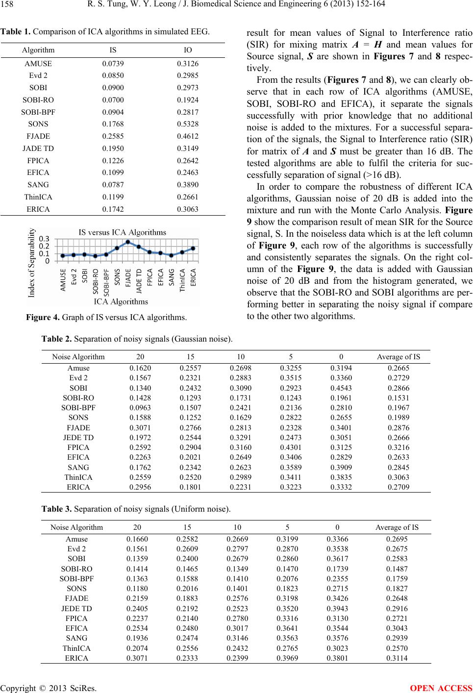 R. S. Tung, W. Y. Leong / J. Biomedical Science and Engineering 6 (2013) 152-164 158 Table 1. Comparison of ICA algorithms in simulated EEG. Algorithm IS IO AMUSE 0.0739 0.3126 Evd 2 0.0850 0.2985 SOBI 0.0900 0.2973 SOBI-RO 0.0700 0.1924 SOBI-BPF 0.0904 0.2817 SONS 0.1768 0.5328 FJADE 0.2585 0.4612 JADE TD 0.1950 0.3149 FPICA 0.1226 0.2642 EFICA 0.1099 0.2463 SANG 0.0787 0.3890 ThinICA 0.1199 0.2661 ERICA 0.1742 0.3063 Figure 4. Graph of IS versus ICA algorithms. result for mean values of Signal to Interference ratio (SIR) for mixing matrix A = H and mean values for Source signal, S are shown in Figures 7 and 8 respec- tively. From the results (Figures 7 and 8), we can clearly ob- serve that in each row of ICA algorithms (AMUSE, SOBI, SOBI-RO and EFICA), it separate the signals successfully with prior knowledge that no additional noise is added to the mixtures. For a successful separa- tion of the signals, the Signal to Interference ratio (SIR) for matrix of A and S must be greater than 16 dB. The tested algorithms are able to fulfil the criteria for suc- cessfully separ a t i o n of signal (>16 dB). In order to compare the robustness of different ICA algorithms, Gaussian noise of 20 dB is added into the mixture and run with the Monte Carlo Analysis. Figure 9 show the comparison result of mean SIR for the Source signal, S. In the noiseless data wh ich is at the left column of Figure 9, each row of the algorithms is successfully and consistently separates the signals. On the right col- umn of the Figure 9, the data is added with Gaussian noise of 20 dB and from the histogram generated, we observe that the SOBI-RO and SOBI algorithms are per- forming better in separating the noisy signal if compare to the other two algorithms. Table 2. Separation of noisy signals (Gaussian noise). Noise Algorithm20151050Average of IS Amuse0.16200.25570.26980.32550.31940.2665 Evd 20.15670.23210.28830.35150.33600.2729 SOBI0.13400.24320.30900.29230.45430.2866 SOBI-RO0.14280.12930.17310.12430.19610.1531 SOBI-BPF0.09630.15070.24210.21360.28100.1967 SONS0.15880.12520.16290.28220.26550.1989 FJADE0.30710.27660.28130.23280.34010.2876 JEDE TD0.19720.25440.32910.24730.30510.2666 FPICA0.25920.29040.31600.43010.31250.3216 EFICA0.22630.20210.26490.34060.28290.2633 SANG0.17620.23420.26230.35890.39090.2845 ThinICA0.25590.25200.29890.34110.38350.3063 ERICA0.29560.18010.22310.32230.33320.2709 Table 3. Separation of noisy signals (Uniform noise). Noise Algorithm20151050Average of IS Amuse0.16600.25820.26690.31990.33660.2695 Evd 20.15610.26090.27970.28700.35380.2675 SOBI0.13590.24000.26790.28600.36170.2583 SOBI-RO0.14140.14650.13490.14700.17390.1487 SOBI-BPF0.13630.15880.14100.20760.23550.1759 SONS0.11800.20160.14010.18230.27150.1827 FJADE0.21590.18830.25760.31980.34260.2648 JEDE TD0.24050.21920.25230.35200.39430.2916 FPICA0.22370.21400.27800.33160.31300.2721 EFICA0.25340.24800.30170.36410.35440.3043 SANG0.19360.24740.31460.35630.35760.2939 ThinICA0.20740.25560.24320.27650.30230.2570 ERICA0.30710.23330.23990.39690.38010.3114 Copyright © 2013 SciRes. OPEN ACCESS  R. S. Tung, W. Y. Leong / J. Biomedical Science and Engineering 6 (2013) 152-164 159 Figure 5. Graph of ISavg versus ICA algorithms in the present of noise (Gaussian noise). Figure 6. Graph of ISavg versus ICA algorithms in the present of noise (Uniform noise). Figure 7. Histogram of SIR for S (sources). Figure 8. Histogram of SIR for A (mixing signals). Copyright © 2013 SciRes. OPEN ACCESS 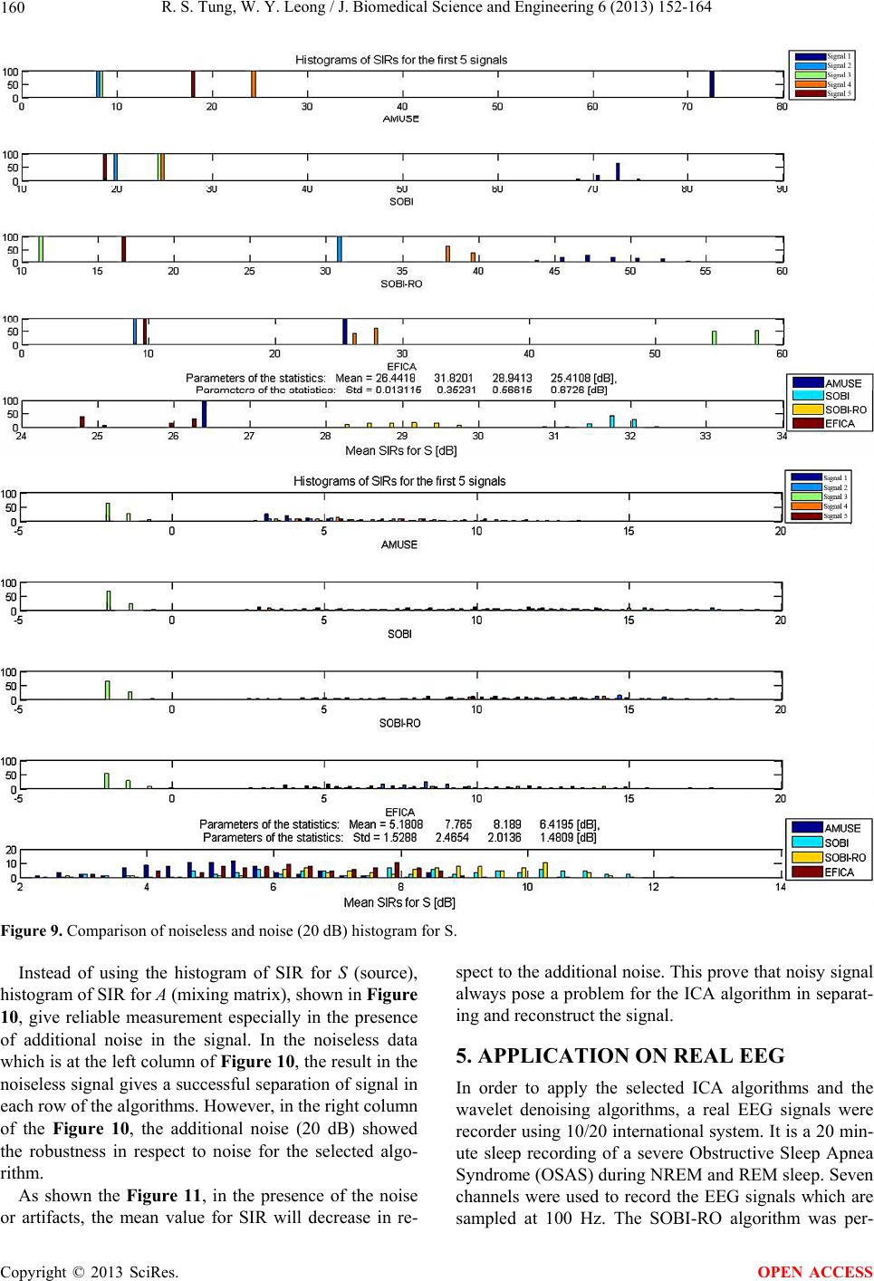 R. S. Tung, W. Y. Leong / J. Biomedical Science and Engineering 6 (2013) 152-164 160 Figure 9. Comparison of noiseless and noise (20 dB) histogram for S. Instead of using the histogram of SIR for S (source), histogram of SIR for A (mixing matrix), shown in Figure 10, give reliable measurement especially in the presence of additional noise in the signal. In the noiseless data which is at the left colu mn of Figure 10, the result in the noiseless signal gives a successful separation of signal in each row of the algorithms. However, in the right column of the Figure 10, the additional noise (20 dB) showed the robustness in respect to noise for the selected algo- rithm. As shown the Figure 11, in the presence of the noise or artifacts, the mean value for SIR will decrease in re- spect to the addition al noise. This prove that noisy signal always pose a problem for the ICA algorithm in separat- ing and reconstruct the signal. 5. APPLICATION ON REAL EEG In order to apply the selected ICA algorithms and the wavelet denoising algorithms, a real EEG signals were recorder using 10/20 international system. It is a 20 min- ute sleep recording of a severe Obstructive Sleep Apnea Syndrome (OSAS) during NREM and REM sleep. Seven channels were used to record the EEG signals which are sampled at 100 Hz. The SOBI-RO algorithm was per- Copyright © 2013 SciRes. OPEN ACCESS 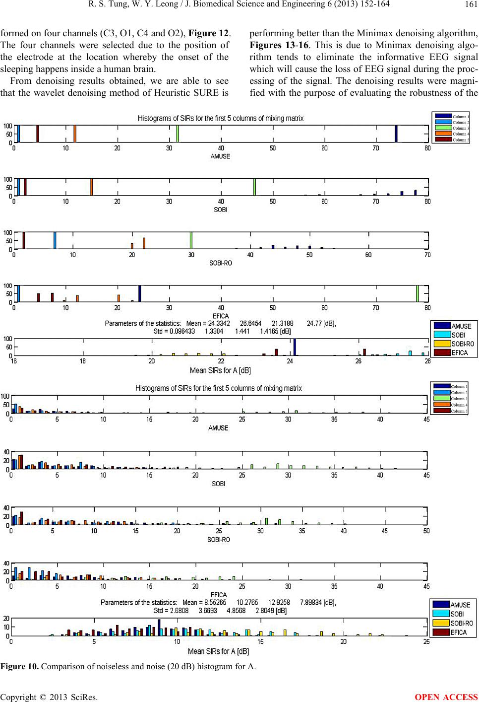 R. S. Tung, W. Y. Leong / J. Biomedical Science and Engineering 6 (2013) 152-164 161 formed on four channels (C3, O1, C4 and O2), Figure 12. The four channels were selected due to the position of the electrode at the location whereby the onset of the sleeping happens inside a human brain. From denoising results obtained, we are able to see that the wavelet denoising method of Heuristic SURE is performing better than the Minimax denoising algorithm, Figures 13-16. This is due to Minimax denoising algo- rithm tends to eliminate the informative EEG signal which will cause the loss of EEG signal during the proc- essing of the signal. The denoising results were magni- fied with the purpose of evaluating the robustness of the Figure 10. Comparison of noiseless and noise (20 dB) histogram for A. Copyright © 2013 SciRes. OPEN ACCESS 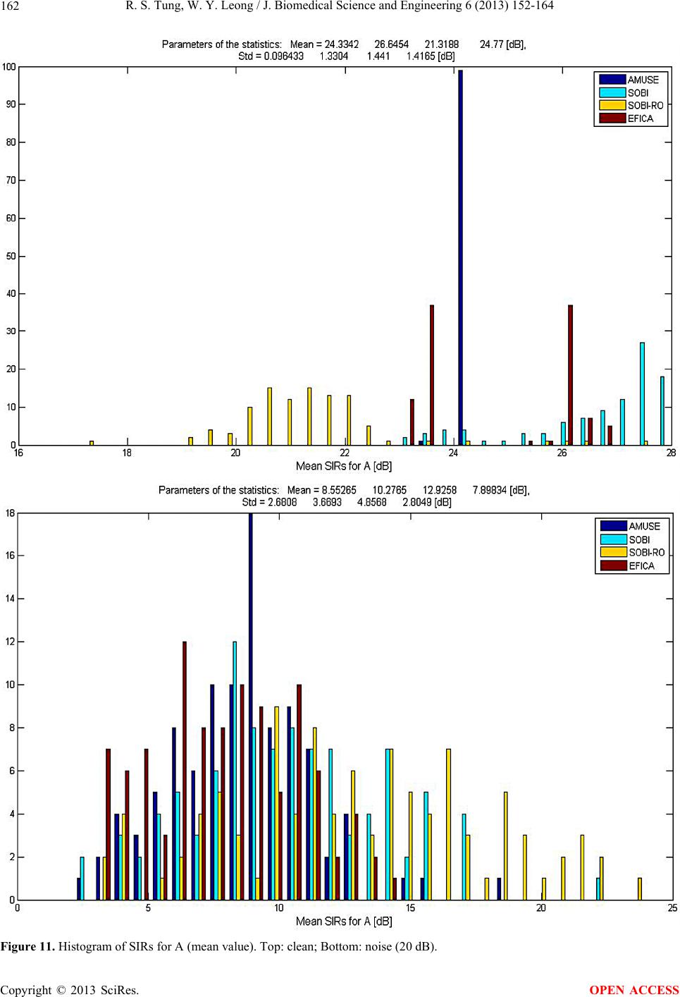 R. S. Tung, W. Y. Leong / J. Biomedical Science and Engineering 6 (2013) 152-164 162 Figure 11. Histogram of SIRs for A (mean value). Top: clean; Bottom: noise (20 dB). Copyright © 2013 SciRes. OPEN ACCESS 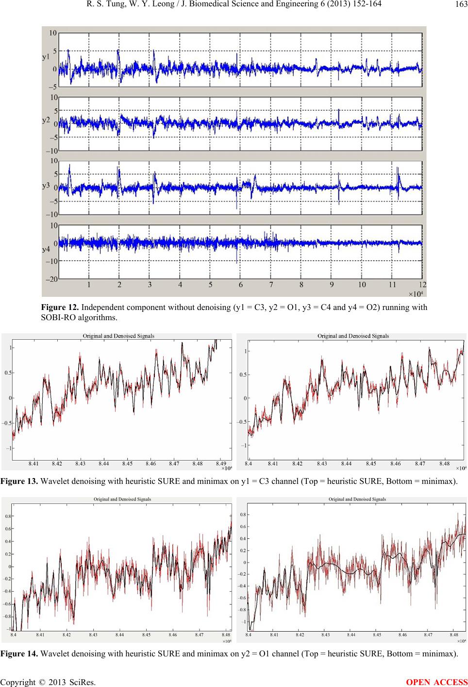 R. S. Tung, W. Y. Leong / J. Biomedical Science and Engineering 6 (2013) 152-164 163 Figure 12. Independent component without denoising (y1 = C3, y2 = O1, y3 = C4 and y4 = O2) running with SOBI-RO algorithms. Figure 13. Wavelet denoising with heuristic SURE and minimax on y1 = C3 channel (Top = heuristic SURE, Bottom = minimax). Figure 14. Wavelet denoising with heuristic SURE and minimax on y2 = O1 channel (Top = heuristic SURE, Bottom = minimax). Copyright © 2013 SciRes. OPEN ACCESS 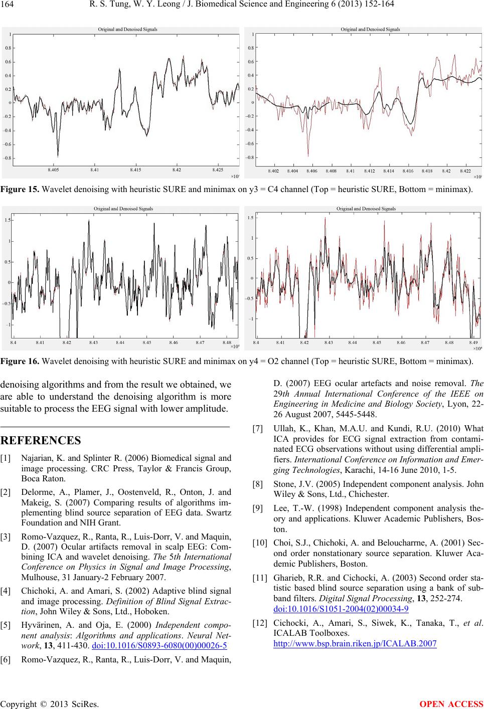 R. S. Tung, W. Y. Leong / J. Biomedical Science and Engineering 6 (2013) 152-164 Copyright © 2013 SciRes. 164 Figure 15. Wavelet denoising with heuristic SURE and minimax on y3 = C4 channel (Top = heuristic SURE, Bottom = minimax). Figure 16. Wavelet denoising with heuristic SURE and minimax on y4 = O2 channel (Top = heuristic SURE, Bottom = minimax). denoising algorithms and from the result we obtained, we are able to understand the denoising algorithm is more suitable to process the EEG signal with lower amplitude. OPEN ACCESS REFERENCES [1] Najarian, K. and Splinter R. (2006) Biomedical signal and image processing. CRC Press, Taylor & Francis Group, Boca Raton. [2] Delorme, A., Plamer, J., Oostenveld, R., Onton, J. and Makeig, S. (2007) Comparing results of algorithms im- plementing blind source separation of EEG data. Swartz Foundation and NIH Grant. [3] Romo-Vazquez, R., Ranta, R., Luis-Dorr, V. and Maquin, D. (2007) Ocular artifacts removal in scalp EEG: Com- bining ICA and wavelet denoising. The 5th International Conference on Physics in Signal and Image Processing, Mulhouse, 31 January-2 February 2007. [4] Chichoki, A. and Amari, S. (2002) Adaptive blind signal and image processing. Definition of Blind Signal Extrac- tion, John Wiley & Sons, Ltd., Hoboken. [5] Hyvärinen, A. and Oja, E. (2000) Independent compo- nent analysis: Algorithms and applications. Neural Net- work, 13, 411-430. doi:10.1016/S0893-6080(00)00026-5 [6] Romo-Vazquez, R., Ranta, R., Luis-Dorr, V. and Maquin, D. (2007) EEG ocular artefacts and noise removal. The 29th Annual International Conference of the IEEE on Engineering in Medicine and Biology Society, Lyon, 22- 26 August 2007, 5445-5448. [7] Ullah, K., Khan, M.A.U. and Kundi, R.U. (2010) What ICA provides for ECG signal extraction from contami- nated ECG observations without using differential ampli- fiers. International Conference on Information and Emer- ging Technologies, Karachi, 14-16 June 2010, 1-5. [8] Stone, J.V. (2005) Independent component analysis. John Wiley & Sons, Ltd., Chichester. [9] Lee, T.-W. (1998) Independent component analysis the- ory and applications. Kluwer Academic Publishers, Bos- ton. [10] Choi, S.J., Chichoki, A. and Beloucharrne, A. (2001) Sec - ond order nonstationary source separation. Kluwer Aca- demic Publishers, Boston. [11] Gharieb, R.R. and Cichocki, A. (2003) Second order sta- tistic based blind source separation using a bank of sub- band filters. Digital Signal Processing, 13, 252-274. doi:10.1016/S1051-2004(02)00034-9 [12] Cichocki, A., Amari, S., Siwek, K., Tanaka, T., et al. ICALAB Toolboxes. http://www.bsp.brain.riken.jp/ICALAB.2007
|