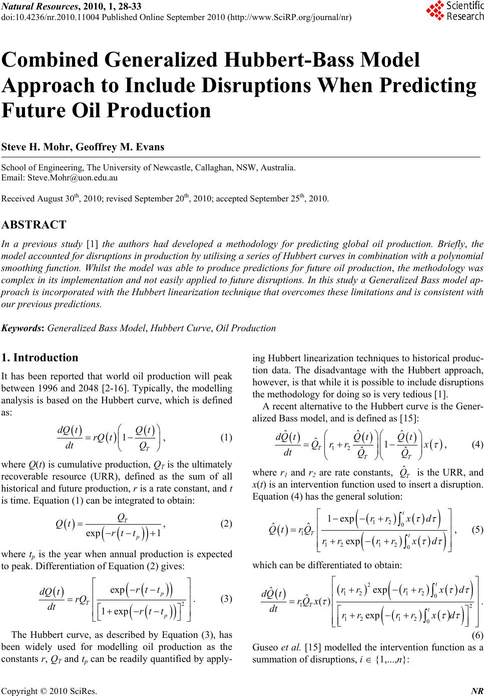Natural Resources, 2010, 1, 28-33
doi:10.4236/nr.2010.11004 Published Online September 2010 (http://www.SciRP.org/journal/nr)
Combined Generalized Hubbert-Bass Model
Approach to Include Disruptions When Predicting
Future Oil Production
Steve H. Mohr, Geoffrey M. Evans
School of Engineering, The University of Newcastle, Callaghan, NSW, Australia.
Received August 30th, 2010; revised September 20th, 2010; accepted September 25th, 2010.
ABSTRACT
In a previous study [1] the authors had developed a methodology for predicting global oil production. Briefly, the
model accounted for disru ptions in p roductio n by u tilising a series of Hubbert curves in comb ination with a polyn omial
smoothing function. Whilst the model was able to produce predictions for future oil production, the methodology was
complex in its implementation and not easily applied to future disrup tions. In this study a Generalized Bass mo del ap-
proach is incorp orated with the Hub bert linearization techn ique that overcomes th ese limitations and is consisten t with
our previous predictions.
Keywords: Generalized Bass Model, Hubbert Curve, Oil Production
1. Introduction
It has been reported that world oil production will peak
between 1996 and 2048 [2-16]. Typically, the modelling
analysis is based on the Hubbert curve, which is defined
as:
  
1
T
dQ tQ t
rQ t
dt Q





, (1)
where Q(t) is cumulative p roduction, QT is the ultimately
recoverable resource (URR), defined as the sum of all
historical and future production, r is a rate constant , and t
is time. Equation (1) can be integrated to obtain:

 
exp 1
T
p
Q
Qt rt t  
, (2)
where tp is the year when annual production is expected
to peak. Differentiation of Equation (2) gives:

 
 
2
exp
1exp
p
T
p
rt t
dQ trQ
dt rt t









. (3)
The Hubbert curve, as described by Equation (3), has
been widely used for modelling oil production as the
constants r, QT and tp can be readily quantified by apply-
ing Hubbert linearization techniques to historical produc-
tion data. The disadvantage with the Hubbert approach,
however, is that while it is possible to include d isruptions
the methodology for doing so is very tedious [1].
A recent alternative to the Hubbert curve is the Gener-
alized Bass model, and is defined as [15]:
 
12
ˆˆˆ
ˆ1
ˆˆ
T
TT
dQ tQ tQ t
Qrr x
dt QQ


 



, (4)
where r1 and r2 are rate constants, is the URR, and
x(t) is an intervention function used to insert a disruption.
Equation (4) has the general solution:
ˆT
Q
 




12
0
1
12 12
0
1exp
ˆˆ
exp
t
Tt
rrx d
QtrQ rrrrx d

















, (5)
which can be differentiated to obtain:
  



2
12 12
0
12
12 12
0
exp
ˆˆ()
exp
t
Tt
rrrrx d
dQ trQ x
dt rrrrx d



























.
(6)
Guseo et al. [15] modelled the intervention function as a
summation of disruptions, i  {1,...,n}: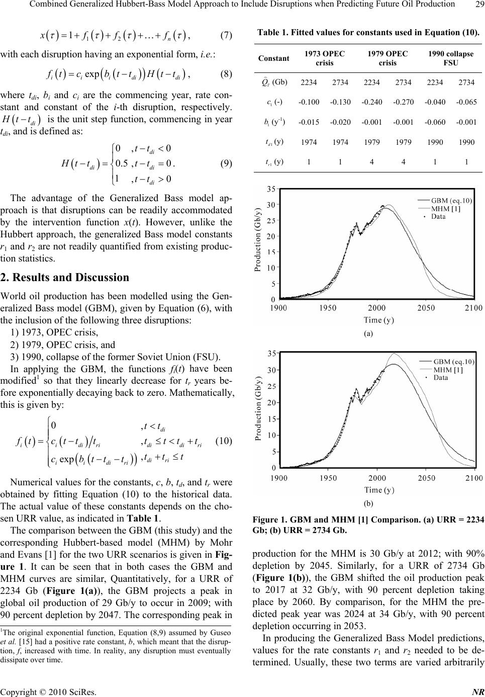

Combined Generalized Hubbert-Bass Model Approach to Include Disruptions when Predicting Future Oil Production29
 


12
1n xff f


    , (7)
with each disruption having an exponential form, i.e.:
 



exp
iiidi

di
f
tc bttHtt

, (8)
where tdi, bi and ci are the commencing year, rate con-
stant and constant of the i-th disruption, respectively.

di
H
tt is the unit step function, commen cing in year
tdi, and is defined as:

0
0.5
1
di
Ht t






,0
,
,0
di
di
di
tt
tt
tt



0
. (9)
The advantage of the Generalized Bass model ap-
proach is that disruptions can be readily accommodated
by the intervention function x(t). However, unlike the
Hubbert approach, the generalized Bass model constants
r1 and r2 are not readily quantif ied from existing produc-
tion statistics.
2. Results and Discussion
World oil production has been modelled using the Gen-
eralized Bass model (GBM), given by Equation (6), with
the inclusion of the following three disruptions:
1) 1973, OPEC crisis,
2) 1979, OPEC crisis, and
3) 1990, collapse of the former Soviet Union (FSU).
In applying the GBM, the functions fi(t) have been
modified1 so that they linearly decrease for tr years be-
fore exponentially decaying back to zero. Mathematically,
this is given by:
 
 
0
exp
iidiri
iidiri
ftctt t
cbttt








,
,
,
di
didi ri
di ri
tt
tttt
ttt

 

(10)
Numerical values for the constants, c, b, td, and tr were
obtained by fitting Equation (10) to the historical data.
The actual value of these constants depends on the cho-
sen URR value, as indicated in Table 1.
The comparison be tween th e GBM (th is study) and th e
corresponding Hubbert-based model (MHM) by Mohr
and Evans [1] for the two URR scenarios is given in Fig-
ure 1. It can be seen that in both cases the GBM and
MHM curves are similar, Quantitatively, for a URR of
2234 Gb (Figure 1(a)), the GBM projects a peak in
global oil production of 29 Gb/y to occur in 2009; with
90 percent depletion by 2047. The corresponding peak in
Table 1. Fitted values for constants used in Equation (10).
Constant 1973 OPEC
crisis 1979 OPEC crisis 1990 collapse FSU
T
Q

(Gb) 223427342234 2734 22342734
1
c(-) -0.100-0.130-0.240 -0.270 -0.040-0.065
1
b(y-1) -0.015-0.020-0.001 -0.001 -0.060-0.001
1d
t(y) 197419741979 1979 19901990
1r
t(y) 1 1 4 4 1 1
(a)
(b)
Figure 1. GBM and MHM [1] Comparison. (a) URR = 2234
Gb; (b) URR = 2734 Gb.
production for the MHM is 30 Gb/y at 2012; with 90%
depletion by 2045. Similarly, for a URR of 2734 Gb
(Figure 1(b)), the GBM shifted the oil production peak
to 2017 at 32 Gb/y, with 90 percent depletion taking
place by 2060. By comparison, for the MHM the pre-
dicted peak year was 2024 at 34 Gb/y, with 90 percent
depletion occ u rri n g i n 2053.
1The original exponential function, Equation (8,9) assumed by Guseo
et al. [15] had a positive rate constant, b, which meant that the disrup-
tion, f, increased with time. In reality, any disruption must eventually
dissipate over time.
In producing the Generalized Bass Model predictions,
values for the rate constants r1 and r2 needed to be de-
termined. Usually, these two terms are varied arbitrarily

Co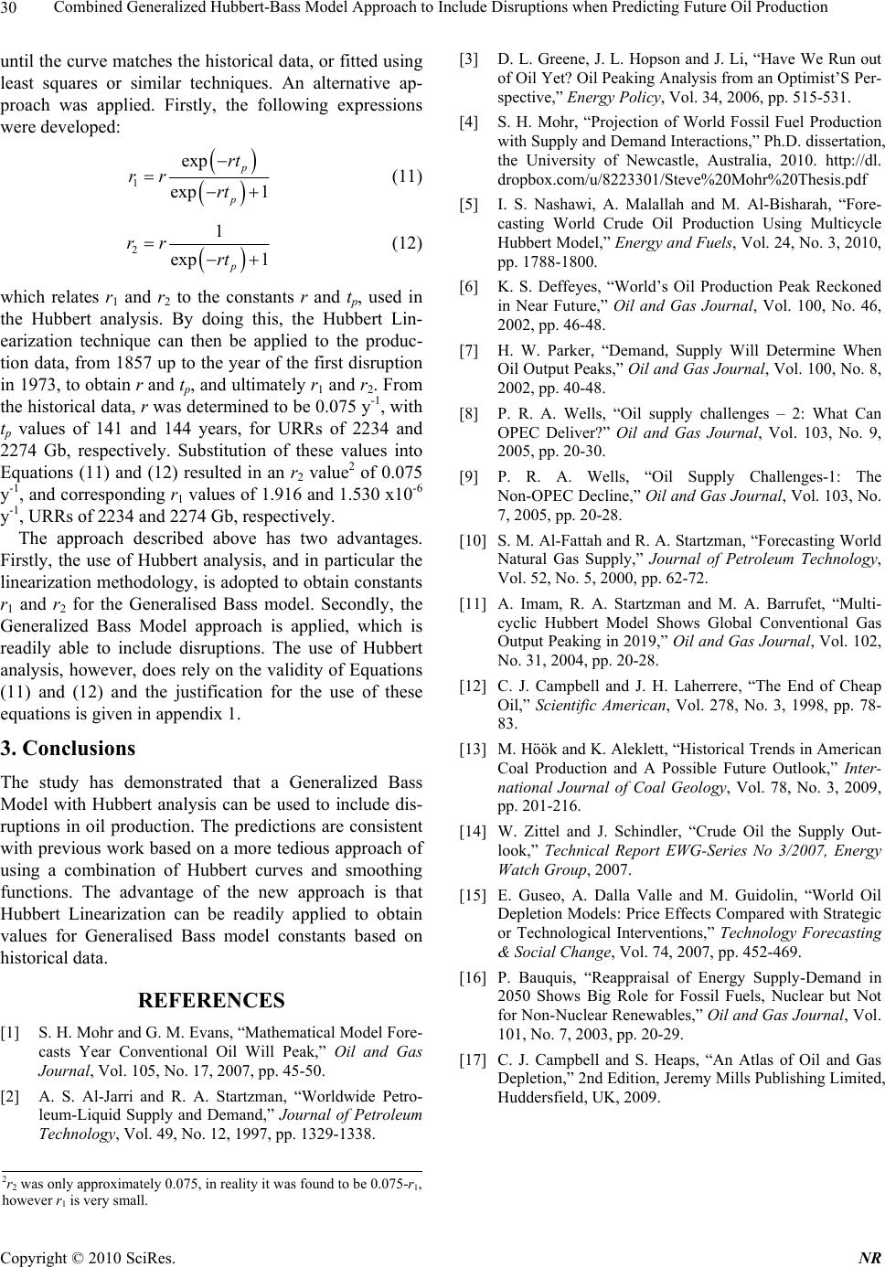mbined Generalized Hubbert-Bass Model Approach to Include Disruptions when Predicting Future Oil Production 30
[3] D. L. Greene, J. L. Hopson and J. Li, “Have We Run out
of Oil Yet? Oil Peaking Analysis from an Optimist’S Per-
spective,” Energy Policy, Vol. 34, 2006, pp. 515-531.
until the curv e matches the historical data, or fitted using
least squares or similar techniques. An alternative ap-
proach was applied. Firstly, the following expressions
were developed: [4] S. H. Mohr, “Projection of World Fossil Fuel Production
with Supply and Demand Interactions,” Ph.D. dissertation,
the University of Newcastle, Australia, 2010. http://dl.
dropbox.com/u/8223301/Steve%20Mohr%20Thesis.pdf


1
exp
exp 1
p
p
rt
rr rt


(11)
[5] I. S. Nashawi, A. Malallah and M. Al-Bisharah, “Fore-
casting World Crude Oil Production Using Multicycle
Hubbert Model,” Energy and Fuels, Vol. 24, No. 3, 2010,
pp. 1788-1800. 
21
exp 1
p
rr rt  (12)
[6] K. S. Deffeyes, “World’s Oil Production Peak Reckoned
in Near Future,” Oil and Gas Journal, Vol. 100, No. 46,
2002, pp. 46-48.
which relates r1 and r2 to the constants r and tp, used in
the Hubbert analysis. By doing this, the Hubbert Lin-
earization technique can then be applied to the produc-
tion data, from 1857 up to the year o f the first disruption
in 1973, to obtain r and tp, and ultimately r1 and r2. From
the historical data, r was determined to be 0.075 y-1, with
tp values of 141 and 144 years, for URRs of 2234 and
2274 Gb, respectively. Substitution of these values into
Equations (11) and (12) resulted in an r2 value2 of 0.075
y-1, and corresponding r1 values of 1.916 an d 1.530 x10-6
y-1, URRs of 2234 and 2274 Gb, respectively.
[7] H. W. Parker, “Demand, Supply Will Determine When
Oil Output Peaks,” Oil and Gas Journal, Vol. 100, No. 8,
2002, pp. 40-48.
[8] P. R. A. Wells, “Oil supply challenges – 2: What Can
OPEC Deliver?” Oil and Gas Journal, Vol. 103, No. 9,
2005, pp. 20-30.
[9] P. R. A. Wells, “Oil Supply Challenges-1: The
Non-OPEC Decline,” Oil and Gas Journal, Vol. 103, No.
7, 2005, pp. 20-28.
The approach described above has two advantages.
Firstly, the use of Hubbert analysis, and in particular the
linearization methodo logy, is adopted to obtain constants
r1 and r2 for the Generalised Bass model. Secondly, the
Generalized Bass Model approach is applied, which is
readily able to include disruptions. The use of Hubbert
analysis, however, does rely on the validity of Equations
(11) and (12) and the justification for the use of these
equations is given in appendix 1.
[10] S. M. Al-Fattah and R. A. Startzman, “Forecasting World
Natural Gas Supply,” Journal of Petroleum Technology,
Vol. 52, No. 5, 2000, pp. 62-72.
[11] A. Imam, R. A. Startzman and M. A. Barrufet, “Multi-
cyclic Hubbert Model Shows Global Conventional Gas
Output Peaking in 2019,” Oil and Gas Journal, Vol. 102,
No. 31, 2004, pp. 20-28.
[12] C. J. Campbell and J. H. Laherrere, “The End of Cheap
Oil,” Scientific American, Vol. 278, No. 3, 1998, pp. 78-
83.
3. Conclusions [13] M. Höök and K. Aleklett, “Historical Trends in American
Coal Production and A Possible Future Outlook,” Inter-
national Journal of Coal Geology, Vol. 78, No. 3, 2009,
pp. 201-216.
The study has demonstrated that a Generalized Bass
Model with Hubbert analysis can be used to include dis-
ruptions in oil production. The predictions are consistent
with previous work based on a more tedious approach of
using a combination of Hubbert curves and smoothing
functions. The advantage of the new approach is that
Hubbert Linearization can be readily applied to obtain
values for Generalised Bass model constants based on
historical da t a .
[14] W. Zittel and J. Schindler, “Crude Oil the Supply Out-
look,” Technical Report EWG-Series No 3/2007, Energy
Watch Group, 2007.
[15] E. Guseo, A. Dalla Valle and M. Guidolin, “World Oil
Depletion Models: Price Effects Compared with Strategic
or Technological Interventions,” Technology Forecasting
& Social Change, Vol. 74, 2007, pp. 452-469.
[16] P. Bauquis, “Reappraisal of Energy Supply-Demand in
2050 Shows Big Role for Fossil Fuels, Nuclear but Not
for Non-Nuclear Renewables,” Oil and Gas Journal, Vol.
101, No. 7, 2003, pp. 20-29.
REFERENCES
[1] S. H. Mohr and G. M. Evans, “Mathematical Model Fore-
casts Year Conventional Oil Will Peak,” Oil and Gas
Journal, Vol. 105, No. 17, 2007, pp. 45-50. [17] C. J. Campbell and S. Heaps, “An Atlas of Oil and Gas
Depletion,” 2nd Edition, Jeremy Mills Publishing Limited,
Huddersfield, UK, 2009.
[2] A. S. Al-Jarri and R. A. Startzman, “Worldwide Petro-
leum-Liquid Supply and Demand,” Journal of Petroleum
Technology, Vol. 49, No. 12, 1997, pp. 1329-1338.
2r2 was only approximately 0.075, in reality it was found to be 0.075-r1,
however r1 is very small.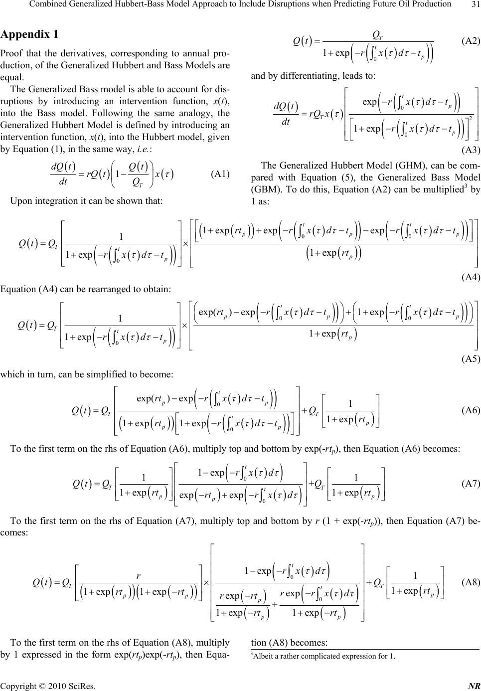

Combined Generalized Hubbert-Bass Model Approach to Include Disruptions when Predicting Future Oil Production31
Appendix 1
Proof that the derivatives, corresponding to annual pro-
duction, of the Generalized Hubbert and Bass Models are
equal.
The Generalized Bass model is able to account for dis-
ruptions by introducing an intervention function, x(t),
into the Bass model. Following the same analogy, the
Generalized Hubbert Model is defined by introducing an
intervention fun ction, x(t), into the Hubbert model, given
by Equation (1), in the same way, i.e.:
  
1
T
dQ tQ t
rQ tx
dt Q





(A1)
Upon integration it can be shown that:
 
 
0
1exp
T
t
p
Q
Qt rx dt


 
 (A2)
and by differentiating, leads to:
  



 
0
2
0
exp
1exp
t
p
Tt
p
rxdt
dQ trQ x
dt rxdt















 










(A3)
The Generalized Hubbert Model (GHM), can be com-
pared with Equation (5), the Generalized Bass Model
(GBM). To do this, Equation (A2) can be multiplied3 by
1 as:
 
 
 






 
 
00
0
1expexpexp
1
1exp
1exp
tt
pp
Ttp
p
rt rxdt rxdt
Qt Qrt
rxdt
 

p





  










 


 


 




(A4)
Equation (A4) can be rearranged to obtain:
 
 









00
0
exp()exp1 exp
1
1exp
1exp
tt
pp
Ttp
p
rtrxdtrxdt
Qt Qrt
rxdt
 

p




  







 


 


 


 




(A5)
which in turn, can be simplified to become:
 







 

0
0
exp() exp1
1exp
1exp 1exp
t
pp
T T
tp
pp
rtr xd t
Qt QQrt
rtr xd t



 





















 (A6)
To the first term on the rhs of Equation (A6), multiply top and bottom by exp(-rtp), then Equation (A6) becomes:









0
0
1exp
11
+
1exp 1exp
exp exp
t
T T
t
p p
p
rx d
Qt QQ
rt rt
rtr xd




 

  

 
 
  



(A7)
To the first term on the rhs of Equation (A7), multiply top and bottom by r (1 + exp(-rtp)), then Equation (A7) be-
comes:

   








0
0
1exp 1
1exp
1 exp1expexp
exp
1 exp1 exp
t
T T
tp
pp p
pp
rx d
r
Qt QQrt
rt rtrrxd
rrt
rt rt





  

 
 

 

 





 



 (A8)
To the first term on the rhs of Equation (A8), multiply
by 1 expressed in the form exp(rtp)exp(-rtp), then Equa-ti on (A 8) bec o mes:
3Albeit a rather complicated expression for 1.

Combined Generalized Hubbert-Bass Model Approach to Include Disruptions when Predicting Future Oil Production 32


  

 

  
 
0
exp exp
1exp 1exp
exp
1exp exp 1exp 1
exp exp
exp
1 exp()1exp exp1exp1
pp
T
pp
t
p
pp
pp
pppp
rtr rt
Qt Qrt rt
rrt rxd
rt rt
rrt rrt
rr
rt rtrt rt

 

 

  
 






  


 








  





0
1
1exp
T
p
t
Qrt
xd 
 
 
 
 

 
 
 

 



 




 


 

(A9)
The first term on the rhs of Equation (A9) is the Gen-
eralised Bass model as expressed in Equation (5). This
can be demonstrated explicitly, by allowing:



exp
ˆ1exp
T
T
p
p
Qrt
Qrt , (A10)


1
exp
exp 1
p
p
rt
rr rt

 , (A11)

21
exp 1
p
rr rt  . (A12)
Substiuting Equation (A10-12) into Equation (A9),
produces:

 





12
0
1
12 12
0
1exp
ˆ
exp
1
1exp
t
Tt
T
p
rrx d
QtQrrrrrx d
Qrt
















 (A13)
Now, the second term on the rhs of Equation (A13) is
the constant4 Q(0), hence Equation (A13) can be rewrit-
ten as:

 

 


12
0
12 12
0
1exp
ˆ0
exp
t
Tt
rrx d
Qt QQ
rrrrx d











.
(A14)
Finally, substitute Equation (5) into Equation (A14) to
obtain:
 
ˆ0QtQtQ . (A15)
Since Q(0) is a constant, differentiating Equation
(A15), leads to:
 
ˆ
dQ tdQ t
dt dt
. (A16)
which shows that the annual production for the General-
ized Hubbert and Bass Models are equal, when the rela-
tionships, given by Equations (A10-12), are applied and
that the cumulative production curves of the Generalized
Hubbert and Bass Models, differ by the constant Q(0).
Note: The Equations (A10-12) can be rearranged to
obtain:
12
rrr

 (A17)


21
12
ln
p
rr
trr  (A18)
(a)
(b)
Figure A1. Comparison between Generalized Bass and
Hubbert models. (a) Annual production; (b) Cumulative
production.
4To see this substitute t = 0 into Equation (A2).

Combined Generalized Hubbert-Bass Model Approach to Include Disruptions when Predicting Future Oil Production33
12
2
ˆ
TT
rr
QQr

 (A19)
The following example is given to demonstrate that
the Generalized Hubbert and Bass models provide
equivalent predictions. Arbitrarily let r = 0.05 y-1, tP =
200 y and QT = 1000 Gb, then from Equation s (A10-12),
r1 = 2.27x10-6 y-1, r2 = 0.05 y-1 and = 999.95 Gb.
Suppose ther e is one disruption in year 150, and that tr =
10 y, c = -0.5 and b= -0.01 y-1. The plots of annual and
cumulative production for both the Generalized Hubbert
and Bass models are shown in Figure A1. It can be seen
that annual production is identical, while the cumulative
production is different only by a constant value of Q(0) =
0.05 Gb.
ˆT
Q