Natural Resources, 2010, 1, 19-27
doi:10.4236/nr.2010.11003 Published Online September 2010 (http://www.SciRP.org/journal/nr)
19
Modeling of Asphaltene Grading in Oil Reservoirs
Julian Y. Zuo1, Oliver C. Mullins2, Chengli Dong3, Dan Zhang1
1DBR Technology Center, Edmonton, Cana da; 2Re servoir Characterization Grou p, Schlumberger, Ho uston, TX, USA; 3North American
Offshore, Schlumberger, Houston, USA.
Received August 10th, 2010; revised September 8th, 2010; accepted September 15th, 2010.
ABSTRACT
Reservoir fluids frequently reveal complex phase behaviors in hydrocarbon columns owing to the effects of gravity,
thermal diffusion, biod egradation, active charging, water washing , seals leaking, and so on. In addition, the formation
compartmentalization often causing discontinuous distributions of fluid compositions and properties makes the proper
fluid characterization and reservoir architecture even more challenging yet compelled. The recognition of composi-
tional grading and flow barriers becomes a key to accurate formation evaluation in a cost effective manner. Downhole
fluid analysis (DFA) of asphaltene gradien ts provides an excellent method to delineate the complexity o f black oil col-
umns. In this paper, a methodology was developed to estimate downhole asphaltene variations with depths using an
equation-of-state (EOS) approach coupled with DFA measurements. DFA tools were used to determine fluid composi-
tions of CO2, C1, C2, C3-C5, C6+, gas-oil ratio (GOR), density and the coloration (optical density) associated with as-
phaltene contents at downhole conditions. The delumping and characterization procedures proposed by Zuo et al.
(2008) were employed to obtain the detailed compositions excluding asphaltenes. In addition, a molar mass distribution
of asphaltene s was described b y a three-p arameter Gamma probab ility function . The Gau ssian quadra ture method wa s
used to generate asphaltene pseudocomponents. Five pseudocomponents were employed to represent the normal as-
phaltene nanoaggregates. Asphaltene distributions in oil columns were computed by tuning the molar mass of asphal-
tene nanoaggregates against the DFA coloration logs at a reference depth. The methodolog y was successfully applied
to investigate black oil reservoir connectivity (or flow barriers) for offshore field cases. The analysis results were con-
sistent with the subsequent production data and analytical chemistry. Furthermore, for simplicity, it is reasonable to
assume that asphaltenes have average properties such as molar mass in entire oil columns. The results obtained in this
work demonstrate that the proposed method provides a useful tool to reduce the uncertainties related to reservoir com-
partmentaliza tion and to optimize the DFA logging during acquisition.
Keywords: Reservoir Connectivity, Asphaltene Gra di ents, Equat i o ns of State, Dow n h ol e F l ui d A nalysis
1. Introduction
In the past few decades, fluid homogeneity has often
been assumed in a reservoir. Reservoir fluids frequently
reveal complex phase behaviors in single oil columns
owing to gravity, thermal gradients, biodegradation, ac-
tive charging, water washing, seals leaking, and so on. In
addition, reservoir compartmentalization often leads to
discontinuous compositional distributions at least of one
fluid analyte, which is the biggest risk factor in deepwa-
ter oil production. A density inversion (higher density
fluids are in the shallower oil column) usually implies a
likely sealing barrier. Knowing actual fluid profiles in the
reservoir enables identification of corresponding com-
partments. Consequently, the family of DFA measure-
ments is expanding in part to enable greater efficacy in
reservoir characterization. Consequently, identifying con-
tinuous fluid gradients in the reservoir provides a method
to suggest connectivity of the reservoir. In particular,
since continuous gradients are generally produced by
time dependent mechanisms, the existence of fluid gra-
dients implies connectivity albeit with an unknown time
scale. Nevertheless, if considerable fluid flow is required
to yield such a gr adien t, this su ggestion of connectiv ity is
much more powerful than that of pressure communica-
tion where little fluid flow is required. In particular, if the
asphaltenes are observ ed to have been equ ilibrated acro ss
a reservoir, laterally and vertically, this is a strong con-
nectivity because 1) asphaltenes necessarily charge into
the reservoir in a much nonequilibrated state and 2) to

Modeling of Asphaltene Grading in Oil Reservoirs 20
equilibrate the component of crude oil with by far the
least mobility necessitates substantial permeability. We
note that measurements of fluid gradients are a far better
way to detect connectivity than measurement of homo-
geneous properties of a fluid. One could easily imagine a
single reservoir charged with a homogeneous fluid,
where the reservoir subsequently develops a sealing bar-
rier either from compaction or faulting . Maintaining con-
tinuous gradients in evolving separate compartments is
much harder to justify. DFA has been used to measure
continuous fluid profiles and stair-step discontinuous
fluid properties addressing reservoir connectivity and
compartmentalization. Fluid compositional variations are
very useful to identify sealing barriers or compartments
in hydrocarbon columns [1,2].
Downhole fluid analysis (DFA) measurements provide
a useful tool to determine the insitu compositional gra-
dients in real time. Recently, Zuo et al. [3] integrated the
equation of state (EOS)-based DFA log predictions with
DFA measurements to delineate the complexity of res-
ervoir fluids and reservoir architecture. This methodol-
ogy is the most suitable for the reservoirs that exhibit
significant compositional grading of at least one chemi-
cal analyte. As mentioned by Hoier and Whitson [4] and
Mullins [5], for equilibrium fluid distribution s, the varia-
tions of fluid compositions and properties are usually
small with depth if the reservoir conditions are far away
from the critical point and the saturation point (e.g.
highly undersaturated black oil). This especially applies
to the alkane distributions [5]. For example, a case study
showed that in an undersaturated black oil reservoir, the
gas-oil ratio (GOR) and compositional gradients were
small for large sand bodies in Gulf of Mexico (GoM)
[1,2]. Nevertheless, the asphaltene gradient was rather
substantial considering the 1000 meters vertical offset of
the tilted sheet reservoir. The flow connectivity in the
reservoir might not be identified according to the infor-
mation of bulk fluids such as compositions, GOR and
density. Fortunately, the DFA tools not only measure
bulk fluid properties like compositions of C1, C2, C3-C5,
C6+ and CO2, GOR and density but also coloration which
is associated with asphaltene contents.
Asphaltenes are defined by a solubility classification,
for example, soluble in toluene, insoluble in n-heptane.
The asphaltenes are the heaviest components of crude
oils with the least diffusivity and have the greatest grad-
ing with depth due to a gravitational force. In the cases
shown by Mullins et al. [1], Betancourt et al. [2] and
Indo et al. [6], the detailed DFA and laboratory analyses
of asphaltene contents indicated the evident asphaltene
gradient with depth while the resin gradients are much
smaller than asphaltenes. The asphaltenes are dispersed
in crude oils as nanoaggregates. This information pro-
vides us a new powerful method of determining flow
connectivity (barriers) in the reservoir by measuring as-
phaltene (coloration) contents with depth at downhole
conditions, especially when bulk fluid property and
compositional gradients are not observable.
Continuous and equilibrium asphaltene gradients have
been observed in deepwater oil fields [1,2,7]. In order to
establish the asphaltene gradient that is in equilibrium, it
is required to establish the co lloidal nature of asphaltenes
in crude oil [1]. It has been established that asphaltenes
are nanocolloidally dispersed in a laboratory setting as
well as a field setting. We note that higher aggregation (a
cluster of nanoaggregates) exists in the reservoir for ei-
ther large asphaltene mass fractions such as heavy oils
and/or unstable crude oils, but there is a class of black
oils with asphaltenes dispersed as ~2nm nanoaggregates.
With this knowledge equilibrium distributions of asphal-
tenes across a field can be established. Asphaltenes in
reservoir crude oils, dispersed as asphaltene nanoaggre-
gates, have by far the lowest rate of diffusion compared
to any crude oil components. Consequently, when they
are in equilibrium throughout a column, then massive
fluid flow is indicated thereby positively constraining
connectivity. Nevertheless, the time frame is still un-
known in these novel analyses. Still the constraint indi-
cates greater connectivity than simply pressure commu-
nication which requires almost no fluid flow at geologi-
cal time scales.
Current DFA tools can measure the coloration of res-
ervoir fluids which is associated with the asphaltene con-
tents. Mullins et al. [1] developed a method to calculate
asphaltene gradient combining DFA data with the
Boltzmann gravitational equation. However, as men-
tioned by Hirschberg [8], the Boltzmann equation is valid
only for ideal solutions. Th e non-ideality should be taken
into account by either the activity coefficient model like
a Flory-Huggins type solubility model or the EOS.
Up to now, no one has applied EOS approach to de-
scribe an asphaltene gradient in reservoirs although there
have been a lot of publications on modeling asphaltene
precipitation (onset) using EOS approach in the open
literature except for work in the references [9]. Following
the traditional EOS approach which has been broadly
used for modeling reservoir fluids, Nghiem et al. [10,11]
arbitrarily split the heaviest component (C31+ fraction) in
the crude oil into two parts: non-precipitating and pre-
cipitating components. The precipitating component was
considered to be an asphaltene component. Qin et al. [12]
implemented the model of Nghiem in their compositional
model. They treated asphaltenes as a pure component
with the same critical properties as heavy hydrocarbons,
except for the binary interaction parameters. Pedersen
and Christensen [13] treated the aromatic fraction of C50+

Modeling of Asphaltene Grading in Oil Reservoirs21
as asphaltenes. The authors mentioned above assumed
that asphaltenes are monomers and part of Cn+ fraction
(e.g, C31+, C36+) in crude oils, which is contradicted with
the recent observations in advanced asphaltene science
that asphaltenes are dispersed as nanoaggregates in crude
oils [1,2,6]. Most recently, the EOS approach was em-
ployed to account for the nonideality of oils [9] and a
methodology for interpreting downhole fluid analysis
was developed for estimating downhole asphaltene varia-
tions with depth. The methodology can be integrated into
the new workflow [3,9,14] as one useful analysis means
in analyzing asphaltene coloration gradients. However,
the EOS approach developed by Zuo et al. [9] treated
asphaltenes to be a single pseudocomponent which is too
simple because asphaltenes are defined as the crude oil
components soluble in toluene but insoluble in n-alkanes
such as n-heptane. The asphaltenes are mixtures which
have components in a wide range of molar masses.
Therefore, distr ibution functio ns and proper char acteriza-
tion of asphaltenes are highly demanding to describe
asphaltene components in the EOS approach.
In this work, the EOS approach was employed to ac-
count for asphaltene gradients in reservoirs. A three-pa-
rameter Gamma distribution function was used to de-
scribe asphaltenes. Two field case studies were presented.
The results in both case studies were proved by the sub-
sequent production data and analytical chemistry. The
results show that the developed methodology can be in-
tegrated into the new workflow [14] as one useful means
in analyzing asphaltene coloration gradients and in dis-
cerning reservoir connectivity.
2. Asphaltene Molar Distributions and
Asphaltene Characterization
Recently, Pomerantz et al. [15] determined molar mass
distributions of asphaltene monomers using two-step
laser mass spectrometry. The results show that petroleum
asphaltenes without aggregation have a peak at every
nominal mass under an envelope beginning at 200 g/mol,
peaking at ~600 g/mol and extending to 1000~1500
g/mol. Mullins et al. [16] reviewed the open literature on
asphaltene molar mass measured by different methods
and concluded that petroleum asphaltenes have a number
average molar mass of ~750 g/mol ( 200 g/mol) with a
range of 500–1,000 g/mol. As mentioned by Mullins in
his new book [17] and the references [1,2], asphaltenes
are dispersed in crude oil as nanoaggregates with 4~10
monomers and ~2 nm in diameter. Hence, the molar
masses of asphaltenes in black oil are in a range of
500–7,500 g/mol from molecules to nanoaggregates
(precluding clusters). On the other hand, asphaltenes may
differ at different depths because asphaltenes are defined
as a solubility class. Therefore, distribu tion functions are
required in characterizing asphaltene components in the
EOS approach because a single component may not be
good enough for asphaltenes.
The three-parameter Gamma function is chosen for
describing molar mass distribution of asphaltene nano-
aggregates [18-20]. Th e pr obab ility d ens ity function , p(x),
is given by
  

1
min min
expxM xM
px





 

 (1)
where
 ,  and Mmin are the three parameters defining the
distribution. Mmin can be set to the average molar mass of
asphaltene monomers [16] for asphaltene nanoaggregates
since it represents the minimum molar mass to be in-
cluded in asphaltene nanoaggregates (e.g., 500 g/mol). If
 is given,  can be estimated by


minavg
MM


 (2)
The parameter  can be determined by fitting experi-
mental data of asphaltene distributions. For most asphal-
tenes and bitumens,  = 3.5 is suitable [21]. Therefore,
the average molar mass of asphaltene nanoaggregates is
only one adjustable parameter in the distributio n function,
which can be determined by matching the DFA color
gradient data in oil columns. The average molar mass of
asphaltene nanoaggregates is adjusted to match DFA
color gradient data (typically, Mavg = ~2,000 g/mol) with
~2 nm in an average diameter.
The Gaussian quadrature method is used to discretize
the continuous Gamma distribution using N quadrature
points [19]. Number of pseudo-components (N) can be
from one to 30 for representing asphaltenes (typically 5).
The asphaltene molar mass distribution function can
be incorporated into the generalized asphaltene gradient
formula described below using the equation of state
(EOS).
3. Generalized Formula for Compositional
and Asphaltene Grading with Depth
Compositional grading in reservoir columns has been
studied by many researchers [3,4,22,23] since 1980s. For
a mixture of reservoir fluids with N-components, a set of
mass flux equations for all components are expressed as
Pr 1,2,..., Chem Grav Thermes
iii ii
J
JJJJi N, (3)
where Ji is the mass flux of component i. The super-
scripts Chem, Grav, Therm and Pres stand for the fluxes
owing to chemical, gravitational, thermal and pressure
forces, respectively.
To calculate compositional gradients with depth in a
hydrocarbon reservoir, it is usually assumed that all the

Modeling of Asphaltene Grading in Oil Reservoirs 22
components of the reservoir fluids have zero mass flux,
which is a stationary state in absence of convection [4].
At the stationary state, the fluxes in Equation (3) are
equal to the external flux at the boundary of the system.
The external flux could be an active charge [22], Jie. It is
assumed that the external mass flux is constant over the
characteristic time scale of filing mechanisms in the for-
mation.
By taking into account the driving forces due to
chemical, gravitational, pressure, thermal impacts and the
external flux, the resulting equations are given by

1,,
0,
1,2,...,
ji
e
NiTi
jii
jjii
TPn
FJRT
nMvg T
nT xD
iN




 





i
(4)
where

i, xi, vi, Mi, Di, g, R,
 and T are the chemical
potential, th e mole fraction, the partial molar volume, the
molar mass and diffusion coefficient of component i, the
gravitational acceleration, universal gas constant, the
density, and the temperature, respectively. FTi is the
thermal diffusion flux of component i and nj is the mole
number of com po nent j.
The thermal diffusion flux of component i (FTi) can be
calculated by the different thermal diffusion models. An
example is the Haase expression [23]
mi
Tii mi
H
H
FM
M
M





(5)
where subscripts m and i stand for the property of the
mixture and component i, respectively. H is the molar
enthalpy. Pedersen and Lindeloff [23] developed expres-
sions for calculating enthalpy. However, the values of
ideal gas enthalpy for C3 and n-C4 are determined by
optimizing absolute ideal gas enthalpy at 273.15 K and
that for C1 was arbitrarily set to zero. The H values can
be treated as adjustable parameters for pseudo-components
to match DFA data in this work. The chemical potential
is calculated through the calculation of fugacity. The
resulting equations are given by

ln 0,
1,2,...,
e
imii
ii
mi ii
Mg hHHJ T
fM
RTMMTx D
iN

 




(6)
where fi is the fugacity of component i and h stands for
the vertical depth. An EOS can be used to estimate the
fugacity of component i.
The critical properties, acentric factors of components
are required for the EOS to calculate fugacity coeffi-
cients. The delumping and characterization procedures of
Zuo and Zhang [24] and Zuo et al. [25] are applied to
characterize single carbon number and plus fractions of
reservoir fluids at a reference depth. The asphaltene
components are characterized by the method described in
the previous section. The EOS is used to estimate fuga-
city. The DFA and/or PVT data are matched by tuning
the EOS parameters to establish a reliable fluid EOS
model. The compositions at depth h are obtained by
solving Equation (6) numerically based on the data at the
reference depth.
In the reference [9], the EOS was used to estimate as-
phaltene grading (profiling) in oil columns. However,
asphaltenes are simply treated to be a single pseu-
docomponent. It is known that asphaltenes are a mixture
whose molar masses vary over a wide range. Therefore,
the asphaltene molar mass distribution function men-
tioned previously is introduced into the EOS approach.
By doing this, everything is kept the same as described in
the reference [9] but asphaltenes are treated as multiple
pseudocomponents using the molar mass distribution
function documented in the previous section to obtain
mole fractions and molar masses.
The properties of the asphaltene pseudocomponents
such as their critical temperatures (Tc) in K, critical pres-
sures (Pc) in atm and acentric factors (  ) are computed
by the correlations in terms of asphaltene molar masses.
It is assumed that asphaltene properties follow the same
trend as the pseudocomponents. The correlations were
then obtained by fitting the pseudocomponent data char-
acterized by the procedures of Zuo and Zhang [24] and
Zuo et al. [25] for more than 10 different crude oils. The
correlation ar e g i v en by
0.2749
53.6746
ci i
PM

 (7)
173.3101ln 439.9450
ci i
TM

 (8)
0.343048ln 1.26763
ii
M


 (9)
The density of asphaltene pseudocomponents in kg/m3
can be calc ul a t e d b y the expression from [26,27]
0.0639
670
ii
M   (10)
where Mi is the molar mass of asphaltene pseudocompo-
nent i. We can also set it as a fixed value of 1200 kg/m3
for all asphaltene pseudocomponents as done by Mullins
[1] and Wang and Buckley [28].
The asphaltene properties are dependent on molar
mass and density just like typical hydrocarbon pseu-
docomponents. The volume translation parameter is es-
timated by matching the specific gravity of asphaltene
components at standard conditions.
4. Results and Discussions
Case 1
The Tahiti field was studied by Betancourt et al. [2] and

Modeling of Asphaltene Grading in Oil Reservoirs23
Mullins et al. [1] using the Boltzmann distribution equa-
tion. The reservoir has a 1,000-m vertical column of
highly undersaturated black oil with GOR in a range of
90 to 116 m3/m3, which slightly decreases with depth.
The formation has two main sands: M21A and M21B,
but are not in pressure communication, so are not in flow
communication. Pressure communication is a necessary
but not su fficient cond ition to establish flow co mmunica-
tion. However, pressure is in communication in each
primary sand body. The case was used to test the meth-
odology proposed in th is work.
The composition (analyzed to C30+) as well as saturate,
aromatics, resin, and asphaltene (SARA) analysis data
were measured at different depths in the laboratory. The
laboratory-measured compositions were then lumped into
the DFA-like five components/groups (CO2, C1, C2,
C3–C5 and C6+, referred to as pseudo-DFA data). The
weight percentages of the five lumped components/
groups were the inputs of the EOS model. The SARA
analysis and the DFA coloration (optical density, OD)
data were applied to determine the relationship between
asphaltene contents in stock-tank oil (STO) and DFA
coloration measured at downhole conditions. The linear
relation was obtained by Betanc ourt et al. [2]: OD = 0.38
 wt% + 0.0059, with a small offset at the origin due to
some coloration of the resin fraction.
Based on the compositions of the five lumped compo-
nents/groups and asphaltene content at a relative depth of
1,555 m in the M21B sand (reference DFA station), as
well as the delumping and characterization method of
Zuo et al. [25], the pseudo-DFA data were delumped and
characterized to full C30+ compositions. The delumped
composition is compared with the gas chromatography
(GC) data as shown in Figure 1. The agreement is good
between the deplumed and GC data. The physical prop-
erties and binary interaction parameters were generated
which are required in the EOS calculation.
Figure 1. Comparison of GC and delumped compositions at
the reference depth for Case 1. The delumped compositions
are in good agreement with the GC data. The delumped
compositions are used as inputs to the asphaltene gradient
analysis.
The predicted phase envelope of this fluid as depicted
in Figure 2 indicates the formation condition is far away
from its critical and bubblepoints (the formation pressure
is ~1400 bar). According to the observation of Hoier and
Whitson [4], it is expected that the fluids have slight
compositional and property grading with depth because
the fluids are hardly compressible and highly undersatu-
rated.
It is assumed that the reservoir is isothermal and there
is no external flux. Compositional gradients with depth
were estimated in terms of the pseudo-DFA data at a
relative depth of 1,555 m (reference depth) by solving
Equation (6) without external fluxes and temperature
gradients. The predicted formation and bubblepoint pres-
sures are compared in Figure 3 with the pretest and
laboratory data. The results show that the predicted for-
mation and bubblepoint pressures agree very well with
the measurements.
Figure 2. Phase envelope for fluid in Case 1. The predicted
bubble point is close to the experimental data. The forma-
tion conditions (P = ~1400 bar) is far away from the critical
and bubble points. Slight compositional gradients are ex-
pected according to the Hoier and Whitson [4] theory.
Figure 3. Comparison of predicted and measured bubble
point and formation pressure for Case 1. The predictions
are in accord with the measurements. The formation pres-
sures are much higher than the bubble points. Slight com-
positional gradients are anticipated according to the Hoier
and Whitson [4] theory.

Modeling of Asphaltene Grading in Oil Reservoirs 24
The predicted compositions are compared with the
measurements as shown in Figure 4. Good agreement is
obtained between the measurements and the predictions.
The compositional gradients of the reservoir fluids
with depth are small in the Tahiti reservoir. Therefore, it
is difficult to determine whether the fluid is in equilib-
rium or in different compartments using the traditional
compositional grading method [3] because the variation
of bulk fluid properties (except asphaltenes) is not evi-
dent. However, the asphaltene gradient in the column can
be used for determining whether the reservoir is in equi-
librium or is disconnected because asphaltenes are the
heaviest components in crude oil and appear in nanoag-
gregates (<10 monomers). In the equilibrium model, as-
phaltenes have the greatest grading in crude oil owing to
a gravitational segregation, although other components
do not have significant gradient with depth. Furthermore,
asphaltene contents are usually low in crude oil and have
little impact on the bulk fluid properties such as GOR,
light-end composition, and/or density. As viscosity soon
joins the pantheon of DFA measurements, asphaltene
content ca n be cro sscorrelat e d to viscosity.
Since the Tahiti fluids are highly undersaturated black
oil with very high formation pressure (~1400 bar) which
is much greater than asphaltene onset pressure and rela-
tive low asphaltene con tent (<5 wt%), there is no asphal-
tene precipitation/deposition (i.e., asphaltenes are stabi-
lized) at downhole conditions. Therefore, there exist no
clusters of asphaltene nanoaggregates but asphaltene
nanoaggregates. The average molar mass of the asphal-
tene nanoaggregates in the distribution function at the
reference depth was adjusted to match the coloration
variation data measured by DFA. The adjusted average
molar mass of the asphaltene nanoaggregates is 1,602
g/mol corresponding to ~2 nm in diameter.
Figure 5 shows the predicted optical density (OD)
variations and DFA measurements with depth. The re-
sults are similar to those obtained by Betancourt et al. [2]
using the Boltzmann distribution equation. The colora-
tion analyses also indicate that the sands of M21A (cen-
ter), M21A North, and M21B are in different compart-
ments. In the paper of Betancourt et al. [2], detailed dis-
cussions were given with regard to reservoir connectivity
and coloration log predictio ns. Th e ideas are employed in
this work as well.
The same fitted molar mass of the asphaltene nanoag-
gregate component is suitable for the entire reservoir.
This means that asphaltenes have the same average size
in nanoaggregates in the oil column. Most of the data
from the field lies on the theoretical fit curves obtained
from the EOS model of asphaltene nanoaggregates. The
GOR of the crude oil is low so relatively uniform. There-
fore, the entire field has the same asphaltene gradient, but
Figure 4. Compositional variations with depth for Tahiti
fluids in Case 1. The predictions are in good agreement with
the experimental data. The compositional gradients are
small with depth, which has confirmed the Hoier and
Whitson [4] theory.
Figure 5. Optical density variations with depth for Case 1.
The lines denote the EOS calculations using an average
asphaltene molar mass of 1602 g/mol. The symbols stand
for the measurements by Live Fluid Analyzer (LFA). Sand
M21A is disconnected with Sand M21B. Sand M21A North
is not connected with main Sand M21A. The subsequent
production data confirmed that the reser voir connectivity is
implied when the reservoir asphaltenes are in equilibrium.
the north part of M21A has a much lower asphaltene
concentration than the south and centric parts of M21A.
As mentioned by Betancourt et al. [2], after a careful
review of the seismic data, it is plausible that the north
part of M21A is disconn ected from the M21A sand ( cen-
ter). The M21B sand is in a different compartment than
the M21A sands as determined by the formation pressure
gradient and geochemistry fingerprinting of the crude oil
samples; the coloration analysis is consistent in this as-
sessment, as seen in Figure 5. The subsequent produc-
tion data from this field confirmed that the reservoir
connectivity is implied when the reservoir asphaltenes
are in equilibrium.
Case 2
Recently, Betancourt et al. [7] reported that black oil
in a 200-m vertical column was analyzed by DFA and
advanced laboratory analytical chemistry methods. The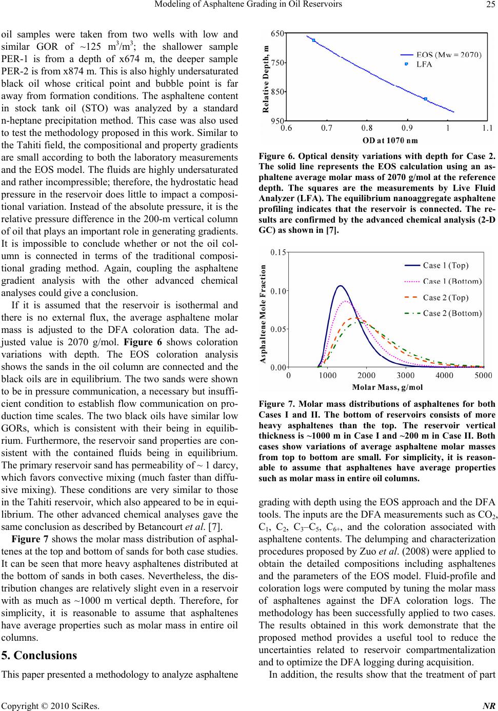

Modeling of Asphaltene Grading in Oil Reservoirs25
oil samples were taken from two wells with low and
similar GOR of ~125 m3/m3; the shallower sample
PER-1 is from a depth of x674 m, the deeper sample
PER-2 is from x874 m. This is also highly undersaturated
black oil whose critical point and bubble point is far
away from formation conditions. The asphaltene content
in stock tank oil (STO) was analyzed by a standard
n-heptane precipitation method. This case was also used
to test the methodology propo sed in this work. Similar to
the Tahiti field, the compositio nal and property gradients
are small according to both the laboratory measurements
and the EOS model. The fluids are highly undersaturated
and rather incompressible; therefore, the hydrostatic head
pressure in the reservoir does little to impact a composi-
tional variation. Instead of the absolute pressure, it is the
relative pressure difference in the 200-m vertical column
of oil that plays an important role in generating gradients.
It is impossible to conclude whether or not the oil col-
umn is connected in terms of the traditional composi-
tional grading method. Again, coupling the asphaltene
gradient analysis with the other advanced chemical
analyses could give a conclusion.
If it is assumed that the reservoir is isothermal and
there is no external flux, the average asphaltene molar
mass is adjusted to the DFA coloration data. The ad-
justed value is 2070 g/mol. Figure 6 shows coloration
variations with depth. The EOS coloration analysis
shows the sands in the oil column are connected and the
black oils are in equilibrium. The two sands were shown
to be in pressure communication, a necessary but insuffi-
cient condition to establish flow communication on pro-
duction time scales. The two black oils have similar low
GORs, which is consistent with their being in equilib-
rium. Furthermore, the reservoir sand properties are con-
sistent with the contained fluids being in equilibrium.
The primar y reserv o i r sa n d h as permeabi l it y of ~ 1 darcy,
which favors convective mixing (much faster than diffu-
sive mixing). These conditions are very similar to those
in the Tahiti reservoir, wh ich also appeared to be in equ i-
librium. The other advanced chemical analyses gave the
same conclusion as described by Betancourt et al. [7].
Figure 7 shows the molar mass distribution of asphal-
tenes at the top and bottom of sands for both case studies.
It can be seen that more heavy asphaltenes distributed at
the bottom of sands in both cases. Nevertheless, the dis-
tribution changes are relatively slight even in a reservoir
with as much as ~1000 m vertical depth. Therefore, for
simplicity, it is reasonable to assume that asphaltenes
have average properties such as molar mass in entire oil
columns.
5. Conclusions
This paper presented a methodology to analyze asphaltene
Figure 6. Optical density variations with depth for Case 2.
The solid line represents the EOS calculation using an as-
phaltene average molar mass of 2070 g/mol at the reference
depth. The squares are the measurements by Live Fluid
Analyzer (LFA). The equilibrium nanoaggregate asphaltene
profiling indicates that the reservoir is connected. The re-
sults are confirmed by the advanced chemical analysis (2-D
GC) as shown in [7].
Figure 7. Molar mass distributions of asphaltenes for both
Cases I and II. The bottom of reservoirs consists of more
heavy asphaltenes than the top. The reservoir vertical
thickness is ~1000 m in Case I and ~200 m in Case II. Both
cases show variations of average asphaltene molar masses
from top to bottom are small. For simplicity, it is reason-
able to assume that asphaltenes have average properties
such as molar mass in entire oil columns.
grading with depth using the EOS approach and the DFA
tools. The inputs are th e DFA measurements such as CO2,
C1, C2, C3–C5, C6+, and the coloration associated with
asphaltene contents. The delumping and characterization
procedures proposed by Zuo et al. (2008) were applied to
obtain the detailed compositions including asphaltenes
and the parameters of the EOS model. Fluid-profile and
coloration logs were computed by tuning the molar mass
of asphaltenes against the DFA coloration logs. The
methodology has been successfully applied to two cases.
The results obtained in this work demonstrate that the
proposed method provides a useful tool to reduce the
uncertainties related to reservoir compartmentalization
and to optimize the DFA logging during acquisition.
In addition, the results show that the treatment of part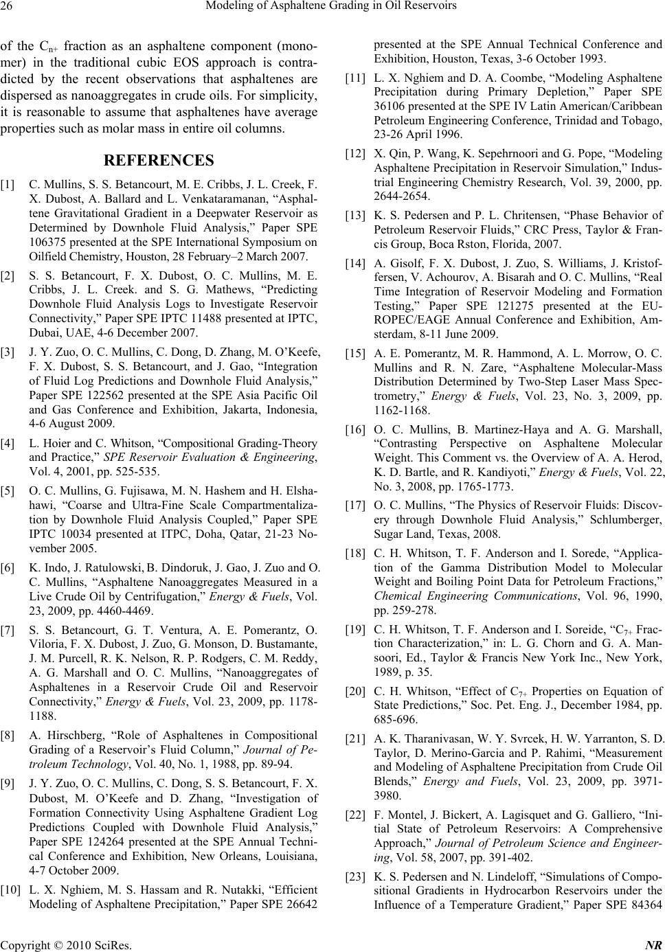

Modeling of Asphaltene Grading in Oil Reservoirs 26
of the Cn+ fraction as an asphaltene component (mono-
mer) in the traditional cubic EOS approach is contra-
dicted by the recent observations that asphaltenes are
dispersed as nanoaggregates in crude oils. For simplicity,
it is reasonable to assume that asphaltenes have average
properties such as molar mass in entire oil columns.
REFERENCES
[1] C. Mullins, S. S. Betancourt, M. E. Cribbs, J. L. Creek, F.
X. Dubost, A. Ballard and L. Venkataramanan, “Asphal-
tene Gravitational Gradient in a Deepwater Reservoir as
Determined by Downhole Fluid Analysis,” Paper SPE
106375 presented at the SPE International Symposium on
Oil f i e l d Chemi s tr y , Hou s to n, 28 F e b r u a r y– 2 Marc h 2007.
[2] S. S. Betancourt, F. X. Dubost, O. C. Mullins, M. E.
Cribbs, J. L. Creek. and S. G. Mathews, “Predicting
Downhole Fluid Analysis Logs to Investigate Reservoir
Connectivity,” Paper SPE IPTC 11488 presented at IPTC,
Dubai, UAE, 4-6 December 2007.
[3] J. Y. Zuo, O. C. Mullins, C. Dong, D. Zhang, M. O’Keefe,
F. X. Dubost, S. S. Betancourt, and J. Gao, “Integration
of Fluid Log Predictions and Downhole Fluid Analysis,”
Paper SPE 122562 presented at the SPE Asia Pacific Oil
and Gas Conference and Exhibition, Jakarta, Indonesia,
4-6 August 2009.
[4] L. Hoier and C. Whitson, “Compositional Grading -The ory
and Practice,” SPE Reservoir Evaluation & Engineering,
Vol. 4, 2001, pp. 525-535.
[5] O. C. Mullins, G. Fujisawa, M. N. Hashem and H. Elsha-
hawi, “Coarse and Ultra-Fine Scale Compartmentaliza-
tion by Downhole Fluid Analysis Coupled,” Paper SPE
IPTC 10034 presented at ITPC, Doha, Qatar, 21-23 No-
vember 2005.
[6] K. Indo, J. Ratulowski, B. Dindoruk, J. Gao, J. Zuo and O.
C. Mullins, “Asphaltene Nanoaggregates Measured in a
Live Crude Oil by Centrifugation,” Energy & Fuels, Vol.
23, 2009, pp. 4460-4469.
[7] S. S. Betancourt, G. T. Ventura, A. E. Pomerantz, O.
Viloria, F. X. Dubost, J. Zuo, G. Monson, D. Bustamante,
J. M. Purcell, R. K. Nelson, R. P. Rodgers, C. M. Reddy,
A. G. Marshall and O. C. Mullins, “Nanoaggregates of
Asphaltenes in a Reservoir Crude Oil and Reservoir
Connectivity,” Energy & Fuels, Vol. 23, 2009, pp. 1178-
1188.
[8] A. Hirschberg, “Role of Asphaltenes in Compositional
Grading of a Reservoir’s Fluid Column,” Journal of Pe-
troleum Technology, Vol. 40, No. 1, 1988, pp. 89-94.
[9] J. Y. Zuo, O. C. Mullins, C. Dong, S. S. Betancourt, F. X.
Dubost, M. O’Keefe and D. Zhang, “Investigation of
Formation Connectivity Using Asphaltene Gradient Log
Predictions Coupled with Downhole Fluid Analysis,”
Paper SPE 124264 presented at the SPE Annual Techni-
cal Conference and Exhibition, New Orleans, Louisiana,
4-7 October 2009.
[10] L. X. Nghiem, M. S. Hassam and R. Nutakki, “Efficient
Modeling of Asphaltene Precipitation,” Paper SPE 26642
presented at the SPE Annual Technical Conference and
Exhibition, Houston, Texas, 3-6 October 1993.
[11] L. X. Nghiem and D. A. Coombe, “Modeling Asphaltene
Precipitation during Primary Depletion,” Paper SPE
36106 presented at the SPE IV Latin American/Caribbean
Petroleum Engineering Conference, Trinidad and Tobago,
23-26 April 1996.
[12] X. Qin, P. Wang, K. Sepehrnoori and G. Pope, “Modeling
Asphaltene Precipitation in Reservoir Simulation,” Indus-
trial Engineering Chemistry Research, Vol. 39, 2000, pp.
2644-2654.
[13] K. S. Pedersen and P. L. Chritensen, “Phase Behavior of
Petroleum Reservoir Fluids,” CRC Press, Taylor & Fran-
cis Group, Boca Rston, Florida, 2007.
[14] A. Gisolf, F. X. Dubost, J. Zuo, S. Williams, J. Kristof-
fersen, V. Achourov, A. Bisarah and O. C. Mullins, “Real
Time Integration of Reservoir Modeling and Formation
Testing,” Paper SPE 121275 presented at the EU-
ROPEC/EAGE Annual Conference and Exhibition, Am-
sterdam, 8-11 June 2009.
[15] A. E. Pomerantz, M. R. Hammond, A. L. Morrow, O. C.
Mullins and R. N. Zare, “Asphaltene Molecular-Mass
Distribution Determined by Two-Step Laser Mass Spec-
trometry,” Energy & Fuels, Vol. 23, No. 3, 2009, pp.
1162-1168.
[16] O. C. Mullins, B. Martinez-Haya and A. G. Marshall,
“Contrasting Perspective on Asphaltene Molecular
Weight. This Comment vs. the Overview of A. A. Herod,
K. D. Bartle, and R. Kandiyoti,” Energy & Fuels, Vol. 22,
No. 3, 2008, pp. 1765-1773.
[17] O. C. Mullins, “The Physics of Reservoir Fluids: Discov-
ery through Downhole Fluid Analysis,” Schlumberger,
Sugar Land, Texas, 2008.
[18] C. H. Whitson, T. F. Anderson and I. Sorede, “Applica-
tion of the Gamma Distribution Model to Molecular
Weight and Boiling Point Data for Petroleum Fractions,”
Chemical Engineering Communications, Vol. 96, 1990,
pp. 259-278.
[19] C. H. Whitson, T. F. Anderson and I. Soreide, “C7+ Frac-
tion Characterization,” in: L. G. Chorn and G. A. Man-
soori, Ed., Taylor & Francis New York Inc., New York,
1989, p. 35.
[20] C. H. Whitson, “Effect of C7+ Properties on Equation of
State Predictions,” Soc. Pet. Eng. J., December 1984, pp.
685-696.
[21] A. K. Tharanivasa n, W. Y. Sv rcek, H. W. Yarranton, S. D.
Taylor, D. Merino-Garcia and P. Rahimi, “Measurement
and Modeling of Asphaltene Precipitation from Crude Oil
Blends,” Energy and Fuels, Vol. 23, 2009, pp. 3971-
3980.
[22] F. Montel, J. Bickert, A. Lagisquet and G. Galliero, “Ini-
tial State of Petroleum Reservoirs: A Comprehensive
Approach,” Journal of Petroleum Science and Engineer-
ing, Vol. 58, 2007, pp. 391-402.
[23] K. S. Pedersen and N. Lindeloff, “Simulations of Compo-
sitional Gradients in Hydrocarbon Reservoirs under the
Influence of a Temperature Gradient,” Paper SPE 84364

Modeling of Asphaltene Grading in Oil Reservoirs 27
presented at the SPE Annual Technical Conference and
Exhibition, Denver, Colorado, 5-8 October 2003.
[24] J. Y. Zuo and D. Zhang, “Plus Fraction Characterization
and PVT Data Regression for Reservoir Fluids near
Critical Conditions,” Paper SPE 64520 presented at the
SPE Asia Pacific Oil and Gas Conference and Exhibition,
Brisbane, Australia, 16-18 October 2000.
[25] J. Y. Zuo, D. Zhang, F. Dubost, C. Dong, O. C. Mullins,
M. O’Keefe and S. S. Betancourt, “EOS-Based Downhole
Fluid Characterization,” Paper SPE 114702 presented at
the SPE Asia Pacific Oil & Gas Conference and Exhibi-
tion, Perth, Australia, 20-22 October 2008.
[26] K. Akbarzadeh, A. Dhillon, W. Y. Svrcek and H. W.
Yarranton, “Methodology for the Characterization and
Modeling of Asphaltene Precipitation from Heavy Oils
Diluted with n-Alkanes,” Energy & Fuels, Vol. 18, 2004,
pp. 1434-1441.
[27] H. Alboudwarej, K. Akbarzadeh, J. Beck, W. Y. Svrcek
and H. W. Yarranton, “Regular Solution Model for As-
phaltene Precipitation from Bitumens and Solvents,”
AIChE Journal, Vol. 49, 2003, pp. 2948-2956.
[28] J. X. Wang and J. S. Buckley, “A Two-Component Solu-
bility Model of the Onset of Asphaltene Flocculation in
Crude Oils,” Energy & Fuels, Vol. 15, 2001, pp. 1004-
1012.