Paper Menu >>
Journal Menu >>
 Natural Resources, 2010, 1, 11-18 doi:10.4236/nr.2010.11002 Published Online September 2010 (http://www.SciRP.org/journal/nr) Copyright © 2010 SciRes. NR 11 Evaluation of Various Linear Regression Methods for Downscaling of Mean Monthly Precipitation in Arid Pichola Watershed Manish Kumar Goyal, Chandra Shekhar Prasad Ojha Dept. of Civil Engineering, Indian Institute of Technology, Roorkee, India. Email: vipmkgoyal@rediffmail.com Received July 20th, 2010; revised August 4th, 2010; accepted August 11th, 2010. ABSTRACT In this paper, downscaling models are developed using various linear regression approaches namely direct, forward, backward and stepwise regression for downscaling of GCM output to predict mean monthly precipitation under IPCC SRES scenarios to watershed-basin scale in an arid region in India. The effectiveness of these regression approaches is evaluated through application to downscale the predictand for the Pichola lake region in Rajasthan state in India, which is considered to be a climatically sensitive region. The predictor variables are extracted from (1) the National Centers for Environmental Prediction (NC E P) reanalysis dataset for the period 1948–2000, and (2) the simulations from the third-generation Canadian Coupled Global Climate Model (CGCM3) for emission scenarios A1B, A2, B1 and COMMIT for the period 2001–2100. The selection of important predictor variables becomes a crucial issue for devel- oping downscaling models since reanalysis data are based on wide range of meteorological measurements and obser- vations. Direct regression was found to yield better performance among all other regression techniques explored in the present study. The results of downscaling models using both approaches show that precipitation is likely to increase in future for A1B, A2 and B1 scenarios, whereas no trend is discerned with the COMMIT. Keywords: Backward, Forward, Precipitation, Regression, Stepwise 1. Introduction Global circulation models (GCMs) are important tool in assessment of climate change. These are numerical mod- els that have been designed to simulate the past, present, and future climate [1]. These models remain relatively coarse in resolution and are unable to resolve significant subgrid scale features. In most climate change impact studies, such as hydrological impacts of climate change, impact models are usually required to simulate sub-grid scale phenomenon and therefore require input data at similar sub-grid scale. The methods used to convert GCM outputs into local meteorological variables re- quired for reliable hydrological modeling are usually referred to as “downscaling” techniques [2,3]. Precipita- tion is an important parameter for climate change impact studies. A proper assessment of probable future precipi- tation and its variability is to be made for various water resources planning and hydro-climatology scenarios. A number of papers have previously reviewed down- scaling concepts, including 1) low-frequency rainfall events [4] 2) daily precipitation [5] 3)seasonal precipita- tion [6] 4) daily and monthly precipitation [7] 5) monthly precipitation [8] 6) monthly precipitation [9] 7) monthly precipitation [10] 8) monthly precipitation [11] 9) annual precipitation [3]. In this paper, we explore four linear regression ap- proaches; namely, (a) direct regression, (b) forward re- gression, (c) backward regression and (d) stepwise re- gression as a downscaling methodology to study climate change impact over Pichola lake basin in an arid region. Apparently, in the literature, there appears no evidence of any study dealing with simultaneous evaluation of vari- ous regression approaches. In the light of this, the objec- tive of this study is to 1) to rank various regression ap- proaches 2) to downscale mean monthly precipitation using best available regression approach from simula- tions of CGCM3 for latest IPCC scenarios. The scenarios which are studied in this paper are relevant to Intergov- ernmental Panel on Climate Change’s (IPCC’s) fourth  Evaluation of Various Linear Regression Methods for Downscaling of 12 Mean Monthly Precipitation in Arid Pichola Watershed assessment report (AR4) which was released in 2007. 2. Study Region The area of the this study is the Pichola lake catchment in Rajasthan in India that is situated from 72.5°E to 77.5°E and 22.5°N to 27.5°N. It receives an average annual pre- cipitation of 597 mm. It has a tropical monsoon climate where most of the precipitation is confined to a few months of the monsoon season. The south–west (summer) monsoon has warm winds blowing from the Indian Ocean causing copious amount of precipitation during June–September months. The Pichola watershed, located in Udaipur district, Rajasthan is one of the major sources for water supply for this arid region. During the past several decades, the streamflow regime in the catchment has changed consid- erably, which resulted in water scarcity, low agriculture yield and degradation of the ecosystem in the study area [12]. Regions with arid and semi-arid climates could be sensitive even to insignificant changes in climatic char- acteristics [13]. Temperature affects the evapotranspira- tion [14], evaporation and desertification processes and is also considered as an indicator of environmental degra- dation and climate change. Understanding the relation- ships among the hydrologic regime, climate factors, and anthropogenic effects is important for the sustainable management of water resources in the entire catchment hence this study area was chosen because of aforemen- tioned reasons. The location map of the study region is shown in Figure 1. 3. Data Extraction The monthly mean atmospheric variables were derived from the National Center for Environmental Prediction (NCEP/NCAR) (hereafter called NCEP) reanalysis data set [15] for a period of January 1948 to December 2000. The data have a horizontal resolution of 2.5° latitude X longitude and seventeen constant pressure levels in ver- tical. The atmospheric variables are extracted for nine grid points whose latitude ranges from 22.5 to 27.5 °N, and longitude ranges from 72.5 to 77.5 °E at a spatial resolution of 2.5°. The precipitation are used at monthly time scale from records available for Pichola Lake which is located in Udaipur at 24° 34’N latitude and 73°40’E longitude. The data is available for the period January 1990 to December 2000 [12].The Canadian Center for Climate Modeling and Analysis (CCCma) provides GCM data for a number of surface and atmospheric variables for the CGCM3 T47 version which has a hori- zontal resolution of roughly 3.75° latitude by 3.75° lon- gitude and a vertical resolution of 31 levels. The data comprise of present-day (20C3M) and future simulations forced by four emission scenarios, namely A1B, A2, B1 and COMMIT. The nine grid points surrounding the study region are selected as the spatial domain of the predictors to adequately cover the various circulation domains of the predictors considered in this study. The GCM data is re-gridded to a common 2.5° using inverse Pichola lake Figure 1. Location map of the study region in Rajasthan State of India with NCEP grid. Copyright © 2010 SciRes. NR  Evaluation of Various Linear Regression Methods for Downscaling of 13 Mean Monthly Precipitation in Arid Pichola Watershed square interpolation technique [16].The utility of this interpolation algorithm was examined in previous down- scaling studies [17,18]. 4. Regression Approaches In statistical methods, the order in which the predictor variables are entered into (or taken out of) the model is determined according to the strength of their correlation with the criterion variable. In direct regression, all available predictor variables are put into the equation at once and they are assessed on the basis of proportion of variances in the criterion vari- able (Y) they uniquely account for. In Forward selection, the variables are entered into the model one at a time in an order determined by the strength of their correlation with the criterion variable. The effect of adding each is assessed as it is entered, and variables that do not significantly add to the success of the model are excluded [19]. In Backward selection, all the predictor variables are entered into the model. The weakest predictor variable is then removed and the regression re-calculated. If this significantly weakens the model then the predictor vari- able is re-entered–otherwise it is deleted. This procedure is then repeated until only useful predictor variables re- main in the model [20,21]. Stepwise is the most sophisticated of these statistical methods. Each variable is entered in sequence and its value assessed. If adding the variable contributes to the model then it is retained, but all other variables in the model are then re-tested to see if they are still contribut- ing to the success of the model. If they no longer con- tribute significantly they are removed. Thus, this method should ensure that one end up with the smallest possible set of predictor variables included in one’s model [22]. 5. Selections of Predictors For downscaling predictand, the selection of appropriate predictors is one of the most important steps in a down- scaling exercise. Various authors have used large-scale atmospheric variables, namely air temperature (at 925, 500 and 200mb pressure levels), geopotential height (at 500 and 200mb pressure levels), zonal (u) and meridional (v) wind velocities (at 925 and 200mb pressure levels), as the predictors for downscaling GCM output to mean monthly precipitation over a catchment [8,10,23]. Predictors have to be selected based both on their rele- vance to the downscaled predictands and their ability to be accurately represented by the GCMs. Cross-correlations are in use to select predictors to understand the presence of nonlinearity/linearity trend in dependence structure [23,24]. These cross-correlations between each of the predictor variables in NCEP and GCM datasets are use- ful to verify if the predictor variables are realistically simulated by the GCM. Cross-correlations are computed between the predictor variables in NCEP and GCM datasets (Table 1). The cross correlations are estimated using three measures of dependence namely, product moment correlation, Spearman’s rank correlation and Kendall’s tau Scatter plots and cross-correlations be- tween each of the predictor variables in NCEP and GCM datasets are useful to verify if the predictor variables are realistically simulated by the GCM. Cross-correlations between each of the predictor variables in NCEP and GCM datasets are useful to verify if the predictor vari- ables are realistically simulated by the GCM. 6. Development of Downscaling Models For downscaling precipitation, the probable predictor variables that have been selected to develop the models are considered at each of the nine grid points surrounding and within the study region. In this study, various linear regression approaches are used to downscale mean monthly precipitation in this study. The data of potential predictors is first standardized. Standardization is widely used prior to statistical downscaling to reduce bias (if any) in the mean and the variance of GCM predictors with respect to that of NCEP-reanalysis data [24]. Standardi- zation is done for a baseline period of 1948 to 2000 be- cause it is of sufficient duration to establish a reliable climatology, yet not too long, nor too contemporary to include a strong global change signal [24]. A feature vector (standardized predictor) is formed for each month of the record using the data of standardized NCEP predictor variables. The feature vector is the input to the linear regression models, and the contemporaneous Table 1. Cross-correlation computed between probable predictors in NCEP and GCM datasets. Ta925 Ua925 Va925 Va200 Ta20 Zg200 Ua200 Ta500 Zg500 P 0.83 0.79 0.67 -0.18 0.66 0.81 0.23 0.81 0.60 S 0.68 0.56 0.43 -0.14 0.46 0.64 0.57 0.64 0.39 K 0.87 0.76 0.61 -0.20 0.68 0.85 0.73 0.85 0.59 H ere P, S and K represent product moment correlation, Spearman’s rank correlation and Kendall’s tau respectively. Copyright © 2010 SciRes. NR 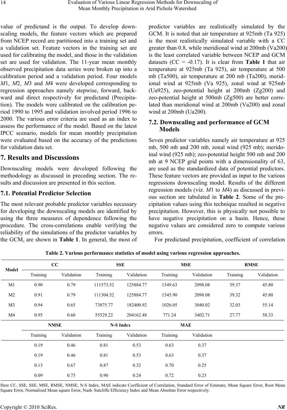 Evaluation of Various Linear Regression Methods for Downscaling of 14 Mean Monthly Precipitation in Arid Pichola Watershed value of predictand is the output. To develop down- scaling models, the feature vectors which are prepared from NCEP record are partitioned into a training set and a validation set. Feature vectors in the training set are used for calibrating the model, and those in the validation set are used for validation. The 11-year mean monthly observed precipitation data series were broken up into a calibration period and a validation period. Four models M1, M2, M3 and M4 were developed corresponding to regression approaches namely stepwise, forward, back- ward and direct respectively for predictand (Precipita- tion). The models were calibrated on the calibration pe- riod 1990 to 1995 and validation involved period 1996 to 2000. The various error criteria are used as an index to assess the performance of the model. Based on the latest IPCC scenario, models for mean monthly precipitation were evaluated based on the accuracy of the predictions for validation data set. 7. Results and Discussions Downscaling models were developed following the methodology as discussed in preceding section. The re- sults and discussion are presented in this section. 7.1. Potential Predictor Selection The most relevant probable predictor variables necessary for developing the downscaling models are identified by using the three measures of dependence following the procedure. The cross-correlations enable verifying the reliability of the simulations of the predictor variables by the GCM, are shown in Table 1. In general, the most of predictor variables are realistically simulated by the GCM. It is noted that air temperature at 925mb (Ta 925) is the most realistically simulated variable with a CC greater than 0.8, while meridional wind at 200mb (Va200) is the least correlated variable between NCEP and GCM datasets (CC = -0.17). It is clear from Table 1 that air temperature at 925mb (Ta 925), air temperature at 500 mb (Ta500), air temperature at 200 mb (Ta200), merid- ional wind at 925mb (Va 925), zonal wind at 925mb (Ua925), zeo-potential height at 200mb (Zg200) and zeo-potential height at 500mb (Zg500) are better corre- lated than meridional wind at 200mb (Va200) and zonal wind at 200mb (Ua200). 7.2. Downscaling and performance of GCM Models Seven predictor variables namely air temperature at 925 mb, 500 mb and 200 mb, zonal wind (925 mb); merido- inal wind (925 mb); zeo-potential height 500 mb and 200 mb at 9 NCEP grid points with a dimensionality of 63, are used as the standardized data of potential predictors. These feature vectors are provided as input to the various regressions downscaling model. Results of the different regression models (viz. M1 to M4) as discussed in previ- ous section are tabulated in Table 2. Some of the pre- cipitation values using this technique resulted in negative precipitation. However, this is physically not possible to have negative precipitation on a basin. Hence, these negative values are considered zero to compute various errors. For predictand precipitation, coefficient of correlation Table 2. Various performance statistics of model using various regression approaches. CC SSE MSE RMSE Model Training Validation Training Validation Training Validation Training Validation M1 0.90 0.79 111573.52 125884.77 1549.63 2098.08 39.37 45.80 M2 0.91 0.79 111304.52 125884.77 1545.90 2098.08 39.32 45.80 M3 0.94 0.65 73875.77 182400.92 1026.05 3040.02 32.03 55.14 M4 0.95 0.60 55529.22 204162.48 771.24 3402.71 27.77 58.33 NMSE N-S Index MAE Training Validation Training Validation Training Validation 0.19 0.46 0.81 0.53 0.63 0.37 0.19 0.46 0.81 0.53 0.63 0.37 0.13 0.67 0.87 0.32 0.70 0.25 0.09 0.75 0.90 0.24 0.72 0.23 Here CC, SSE, SSE, MSE, RMSE, NMSE, N-S Index, MAE indicate Coefficient of Correlation, Standard Error of Estimate, Mean Square Error, Root Mean Square Error, Normalized Mean square Error, Nash–Sutcliffe Efficiency Index and Mean Absolute Error respectively. Copyright © 2010 SciRes. NR  Evaluation of Various Linear Regression Methods for Downscaling of 15 Mean Monthly Precipitation in Arid Pichola Watershed (CC) was in the range of 0.65-0.95, RMSE was in the range of 27.77-58.33, N-S Index was in the range of 0.24-0.90 and MAE was in the range of 0.23-0.72 for regression based models (viz. M1 to M4) for training and validation set. It can be observed from Table 2 that the performance of direct regression models for mean monthly precipitation are clearly superior to that of for- ward, backward and stepwise regression based models in training data set while the performance of stepwise and forward regression models for predictand are clearly su- perior to that of backward and direct regression based models in validation data set. Results of forward and stepwise regression are quite similar. It can be inferred that model M4 using direct regression performed best for predictand precipitation. A comparison of mean monthly observed precipitation with precipitation simulated using forward regression models M4 has been shown from Figure 2 for calibration and validation period. Calibration period is from 1990 to 1995, and the rest is validation period. Once the downscaling models have been calibrated and validated, the next step is to use these models to downscale the control scenario simulated by the GCM. The GCM simulations are run through the calibrated and validated direct regression model M4 to obtain future simulations of predictand. The predictand patterns are analyzed with box plots for 20 year time slices. Typical results of downscaled predictand obtained from the pre- dictors are presented in Figure 3. In part (i) of Figure 3, the precipitation downscaled using NCEP and GCM datasets are compared with the observed precipitation for the study region using box plots. The projected precipita- tion for 2001–2020, 2021–2040, 2041–2060, 2061–2080 and 2081–2100, for the four scenarios A1B, A2, B1 and COMMIT are shown in (ii), (iii), (iv) and (v) respec- tively. From the box plots of downscaled predictand (Figure 3), it can be observed that precipitation are projected to increase in future for A1B, A2 and B1 scenarios. The projected increase of precipitation is high for A1B and A2 scenarios whereas it is least for B1 scenario. This is because among the scenarios considered, the scenario A1B and A2 have the highest concentration of atmos- pheric carbon dioxide (CO2) equal to 720 ppm and 850 ppm, while the same for B1 and COMMIT scenarios are 550 ppm and ≈ 370 ppm respectively. Rise in concentra- tion of CO2 in the atmosphere causes the earth’s average temperature to increase, which in turn causes increase in evaporation especially at lower latitudes. The evaporated water would eventually precipitate [10,25]. In the COMMIT scenario, where the emissions are held the same as in the year 2000, no significant trend in the pat- tern of projected future precipitation could be discerned. The overall results show that the projections obtained for precipitation are indeed robust. 8. Conclusions This paper investigates the applicability of the various linear regression approaches such as direct, forward, backward and stepwise to downscale precipitation from Figure 2. Typical results for comparison of the monthly observed Precipitation with Precipitation simulated using direct re- gression downscaling model M4 for NCEP data. In the Figure calibration period is from 1990 to 1995, and the rest is valida- tion period. Copyright © 2010 SciRes. NR  Evaluation of Various Linear Regression Methods for Downscaling of 16 Mean Monthly Precipitation in Arid Pichola Watershed (a) (b) (c) (d) (e) Figure 3. Box plots results from the direct regression-based downscaling model M4 for the predictand Precipitation. Copyright © 2010 SciRes. NR 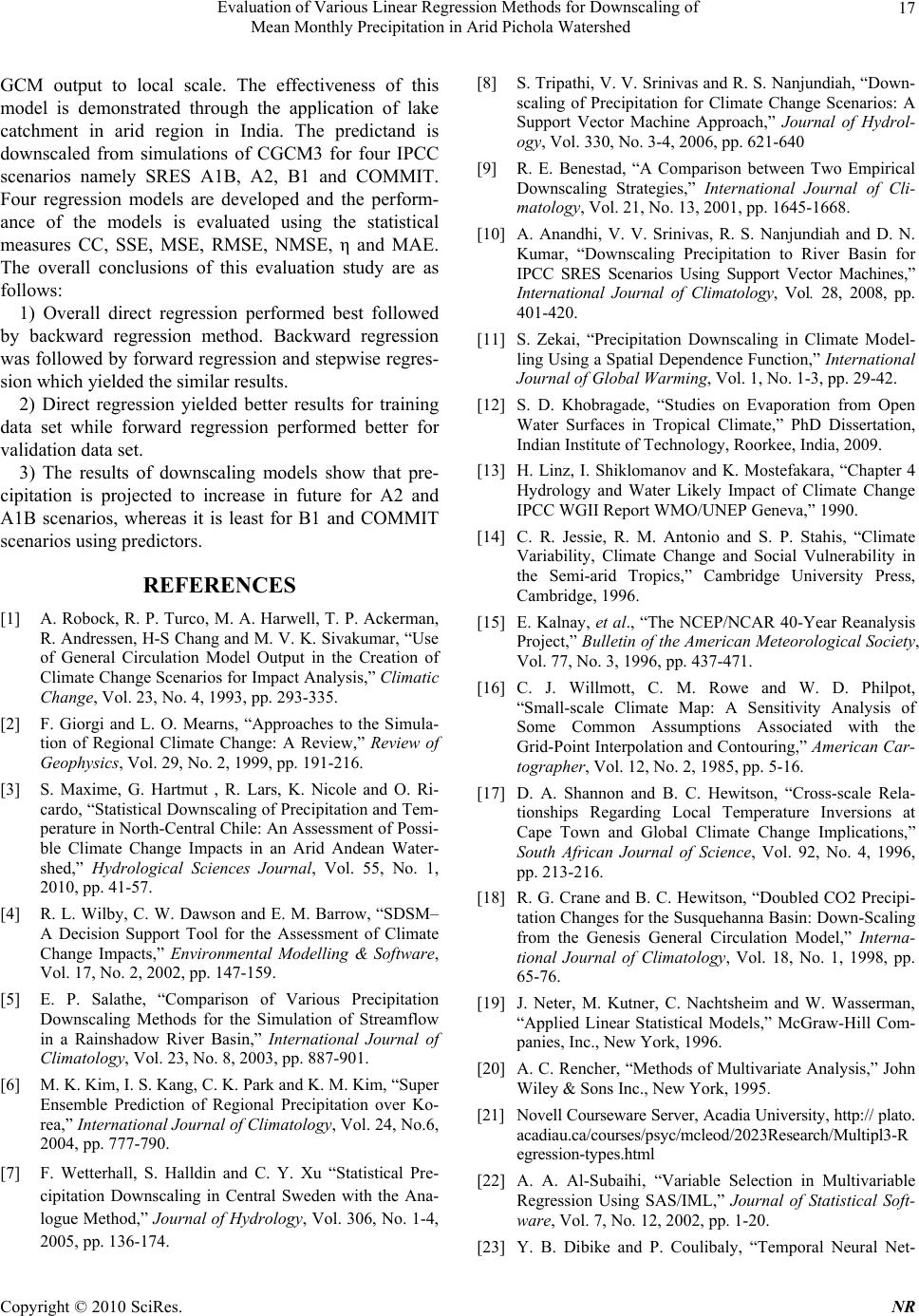 Evaluation of Various Linear Regression Methods for Downscaling of Mean Monthly Precipitation in Arid Pichola Watershed Copyright © 2010 SciRes. NR 17 GCM output to local scale. The effectiveness of this model is demonstrated through the application of lake catchment in arid region in India. The predictand is downscaled from simulations of CGCM3 for four IPCC scenarios namely SRES A1B, A2, B1 and COMMIT. Four regression models are developed and the perform- ance of the models is evaluated using the statistical measures CC, SSE, MSE, RMSE, NMSE, η and MAE. The overall conclusions of this evaluation study are as follows: 1) Overall direct regression performed best followed by backward regression method. Backward regression was followed by forward regression and stepwise regres- sion which yielded the similar results. 2) Direct regression yielded better results for training data set while forward regression performed better for validation data set. 3) The results of downscaling models show that pre- cipitation is projected to increase in future for A2 and A1B scenarios, whereas it is least for B1 and COMMIT scenarios using predictors. REFERENCES [1] A. Robock, R. P. Turco, M. A. Harwell, T. P. Ackerman, R. Andressen, H-S Chang and M. V. K. Sivakumar, “Use of General Circulation Model Output in the Creation of Climate Change Scenarios for Impact Analysis,” Climatic Change, Vol. 23, No. 4, 1993, pp. 293-335. [2] F. Giorgi and L. O. Mearns, “Approaches to the Simula- tion of Regional Climate Change: A Review,” Review of Geophysics, Vol. 29, No. 2, 1999, pp. 191-216. [3] S. Maxime, G. Hartmut , R. Lars, K. Nicole and O. Ri- cardo, “Statistical Downscaling of Precipitation and Tem- perature in North-Central Chile: An Assessment of Possi- ble Climate Change Impacts in an Arid Andean Water- shed,” Hydrological Sciences Journal, Vol. 55, No. 1, 2010, pp. 41-57. [4] R. L. Wilby, C. W. Dawson and E. M. Barrow, “SDSM– A Decision Support Tool for the Assessment of Climate Change Impacts,” Environmental Modelling & Software, Vol. 17, No. 2, 2002, pp. 147-159. [5] E. P. Salathe, “Comparison of Various Precipitation Downscaling Methods for the Simulation of Streamflow in a Rainshadow River Basin,” International Journal of Climatology, Vol. 23, No. 8, 2003, pp. 887-901. [6] M. K. Kim, I. S. Kang, C. K. Park and K. M. Kim, “Super Ensemble Prediction of Regional Precipitation over Ko- rea,” International Journal of Climatology, Vol. 24, No.6, 2004, pp. 777-790. [7] F. Wetterhall, S. Halldin and C. Y. Xu “Statistical Pre- cipitation Downscaling in Central Sweden with the Ana- logue Method,” Journal of Hydrology, Vol. 306, No. 1-4, 2005, pp. 136-174. [8] S. Tripathi, V. V. Srinivas and R. S. Nanjundiah, “Down- scaling of Precipitation for Climate Change Scenarios: A Support Vector Machine Approach,” Journal of Hydrol- ogy, Vol. 330, No. 3-4, 2006, pp. 621-640 [9] R. E. Benestad, “A Comparison between Two Empirical Downscaling Strategies,” International Journal of Cli- matology, Vol. 21, No. 13, 2001, pp. 1645-1668. [10] A. Anandhi, V. V. Srinivas, R. S. Nanjundiah and D. N. Kumar, “Downscaling Precipitation to River Basin for IPCC SRES Scenarios Using Support Vector Machines,” International Journal of Climatology, Vol. 28, 2008, pp. 401-420. [11] S. Zekai, “Precipitation Downscaling in Climate Model- ling Using a Spatial Dependence Function,” International Journal of Global Warming, Vol. 1, No. 1-3, pp. 29-42. [12] S. D. Khobragade, “Studies on Evaporation from Open Water Surfaces in Tropical Climate,” PhD Dissertation, Indian Institute of Technology, Roorkee, India, 2009. [13] H. Linz, I. Shiklomanov and K. Mostefakara, “Chapter 4 Hydrology and Water Likely Impact of Climate Change IPCC WGII Report WMO/UNEP Geneva,” 1990. [14] C. R. Jessie, R. M. Antonio and S. P. Stahis, “Climate Variability, Climate Change and Social Vulnerability in the Semi-arid Tropics,” Cambridge University Press, Cambridge, 1996. [15] E. Kalnay, et al., “The NCEP/NCAR 40-Year Reanalysis Project,” Bulle tin of the American Meteorological Society, Vol. 77, No. 3, 1996, pp. 437-471. [16] C. J. Willmott, C. M. Rowe and W. D. Philpot, “Small-scale Climate Map: A Sensitivity Analysis of Some Common Assumptions Associated with the Grid-Point Interpolation and Contouring,” American Car- tographer, Vol. 12, No. 2, 1985, pp. 5-16. [17] D. A. Shannon and B. C. Hewitson, “Cross-scale Rela- tionships Regarding Local Temperature Inversions at Cape Town and Global Climate Change Implications,” South African Journal of Science, Vol. 92, No. 4, 1996, pp. 213-216. [18] R. G. Crane and B. C. Hewitson, “Doubled CO2 Precipi- tation Changes for the Susquehanna Basin: Down-Scaling from the Genesis General Circulation Model,” Interna- tional Journal of Climatology, Vol. 18, No. 1, 1998, pp. 65-76. [19] J. Neter, M. Kutner, C. Nachtsheim and W. Wasserman, “Applied Linear Statistical Models,” McGraw-Hill Com- panies, Inc., New York, 1996. [20] A. C. Rencher, “Methods of Multivariate Analysis,” John Wiley & Sons Inc., New York, 1995. [21] Novell Courseware Server, Acadia University, http:// plato. acadiau.ca/courses/psyc/mcleod/2023Research/Multipl3-R egression-types.html [22] A. A. Al-Subaihi, “Variable Selection in Multivariable Regression Using SAS/IML,” Journal of Statistical Soft- ware, Vol. 7, No. 12, 2002, pp. 1-20. [23] Y. B. Dibike and P. Coulibaly, “Temporal Neural Net-  Evaluation of Various Linear Regression Methods for Downscaling of 18 Mean Monthly Precipitation in Arid Pichola Watershed works for Downscaling Climate Variability and Ex- tremes,” Neural Networks, Vol. 19, No. 2, 2006, pp. 135- 144. [24] R. L. Wilby, S. P. Charles, E. Zorita, B. Timbal, P. Whet- ton and L. O. Mearns, “The Guidelines for Use of Climate Scenarios Developed from Statistical Downscaling Meth- ods,” p. 27, 2004. http://ipcc-ddc.cru.uea.ac.uk [25] M. K. Goyal and C. S. P. Ojha, “Robust Weighted Re- gression as a Downscaling Tool in Temperature Projec- tions,” International Journal of Global Warming. 2010. http://www.inderscience.com/browse/index.php?journalI D=331 &action=coming Copyright © 2010 SciRes. NR |