Advances in Pure Mathematics, 2013, 3, 159-163
http://dx.doi.org/10.4236/apm.2013.31A022 Published Online January 2013 (http://www.scirp.org/journal/apm)
Numerical Solutions of the Regularized Long-Wave
(RLW) Equation Using New Modification of
Laplace-Decomposition Method
Nawal A. Al-Zaid, Huda O. Bakodah, Fathiah A. Hendi
Department of Mathematics, Science Faculty for Girls, King Abdulaziz University, Jeddah, KSA
Received July 28, 2012; revised September 30, 2012; accepted October 8, 2012
ABSTRACT
In this paper the new modification of Laplace Adomian decomposition method (ADM) to obtain numerical solution of
the regularized long-wave (RLW) equation is presented. The performance of the method is illustrated by solving two
test examples of the problem. To see the accuracy of the method, L2 and L∞ error norms are calculated.
Keywords: Adomian Decomposition Method; Regularized Long-Wave (RLW); Laplace Transform
1. Introduction
The regularized long wave (RLW) equation which can be
shown in the form
0
txx xxt
uu uuu

 

(1)
where ,

are positive parameters, is an important
nonlinear wave equation. This equation plays a major
role in the study of nonlinear dispersive waves. The
RLW equation particularly describes the behavior of the
undular bore [1-3], it has also been derived from the
study of water waves and ion acoustic plasma waves.
The RLW equation has been solved analytically only
for restricted set of boundary and initial conditions. There-
fore, the numerical solution of this equation has been the
subject of many papers [4-7]. Recently a great deal of
interest has been focused on application of Adomian de-
composition method (ADM) to solve a wide variety of
nonlinear problems [8,9]. In this paper, we will apply the
new modification of Laplace ADM to the RLW Equation
(1). The soliton solution of RLW equation has the form





2
0
sech px vtx, 3uxt c (2)
where is an arbitrary constant and
p

1
2
21
c
c 





1vc 1
1
p,
,

0
 
,0uxf x

, and c is a constant [10]. In this
work, a new modification of Laplace ADM is used to
solve the RLW equation with the initial condition
(3)
x is a localized disturbance inside the con-
sidered interval.
where
2. Description of Method
We begin by consider Equation (1) in an operator form


0
tx
LuuRuNu 
f

 (4)
where t
Lt






is a linear operator and R its remainder
of the linear operator. The nonlinear term is represented
by


Nu
 
tx
LuuR uNu   
 
0
,,
n
n
uxtu xt



0
. Thus we get
(5)
We represent solution as an infinite series given be-
low,
(6)
The nonlinear term Nu can be decomposed into infi-
nite series of polynomial given by:
x
n
n
Nu uuA




,, ,
n
uu u
000
10110
2021120
x
xx
xxx
Auu
Auuuu
(7)
where An are Adomian polynomials [11] of 01
and it can be calculated by formula given below:
uuuu uu




A
and so on. The rest of the polynomials can be constructed
C
opyright © 2013 SciRes. APM

N. A. AL-ZAID ET AL.
160
in a similar manner.
By applying the Laplace transform to both sides of
Equation (5), we obtain
 

tx
Lu u   
 
Ru Nu (8)
Thus
  


11
,,0
x
uxt uxuR
  
u Nu
s
s
 
(9)
In the new modification of ADM [12], Wazwaz re-
placed the initial condition


,0ux

0,
0n
n
u x



by a series of infi-
nite components i.e.,

,0ux (10)
and the new recursive relationship can be expressed in
the form
 
 
 
0 0,0
10,1
1
,,0,
1
,,0
1
nn
x
Uxsu x
s
Uxs ux
s
uRu
 
,0 Nun
s




    

0
,
n
n
U xs



(11)
where
  
,,uxt Uxs (12)
Now, by applying inverse Laplace transformation we
get:




 
,, ,0
xs
xsn
m
u

0
,
m
mi
i
uuxt


u e

1
00
1
11
,,
nn
uxt U
uxtU




 (13)
Using (13) the series solution follows immediately.
3. Numerical Examples and Results
In this section, the new modification of Laplace ADM
will be demonstrated on illustrative examples and we
compare the approximate solution obtained for our RLW
equation with known exact solutions. We define to be
m-term approximate solution, i.e.
e the exact solution and m the absolute error between
the exact solution and the approximate solution
mem
euu
In order to show how good the numerical solutions are
in comparison with the exact ones, we will use the L2 and
L∞ error norms defined by
1
2
2
22 ,,
1
m
em eimi
i
Luuxu u



 





,,
max
em eimi
i
Luu uu

Example (1)
We consider Equation (1) with the initial condition
 



2
0
,03 sechuxcpx x
The exact solution of this problem is given by Equation
(2). This solution corresponds to the motion of a single
solitary wave with amplitude 3c and width p, initially
centered at 0
x
, where 1vc


1
is the wave velocity. We
use the new modification of Laplace ADM to solve this
equation, all computations are done for the parameters
00x

,

1


and

.
0.1cWe consider

, as in [13], so the initial condition


,0ux can expressed as a series of infinite components
i.e.



24
12
68 10
,00.3 0.006818180.000103306
1.330451.5754 1.77355
uxx x
x
xxOx
 
 
  
Using recursive relation (11) yield the components
11
00
0.3
,, 0.3
uxt Uxss






  
11 2
11
2
0.00681818
,,
0.00681818
uxt Uxsx
s
x












 
1
22
4
,,
0.0177273 0.000103306
uxtUxs
tx x











1
33
23
66
,,
0.0115227 0.000630165
1.3304510
uxt Uxs
ttx
x



 


And so on, in this manner the rest of components of
the decomposition series were obtained. The results are
given in Table 1. The error norms for (c = 0.1) are re-
corded in Table 2 for different value of m.
Also in Figure 1 we show the exact solution and nu-
merical solution with new modification of Laplace ADM
for t = 0.1 and t = 0.5. Figure 2 shows the exact solution
and numerical solution with new modification for t = 0.5
at the interval 5 ≤ x ≤ 5.
Example (2)
In the second test problem [14], a smaller solitary wave
of amplitude 0.109 (c = 0.05), has been modeled.

The initial condition

,0ux can expressed as a se-
ies of infinite components i.e. r

N. A. AL-ZAID ET AL.
161
Table 1. Absolute errors for Example (1) with c = 0.1 and m = 10.
x/t 0.01 0.02 0.03 0.04 0.05
0.1 4.60152 × 10−7 4.29123 × 10−7 9.14459 × 10−8 1.09975 × 10−6 2.59382 × 10−6
0.2 1.15346 × 10−6 1.8112 × 10−6 1.97626 × 10−6 1.65183 × 10−6 8.41272 × 10−7
0.3 1.82435 × 10−6 3.1446 × 10−6 3.96518 × 10−6 4.29071 × 10−6 4.12595 × 10−6
0.4 2.4624 × 10−6 4.40862 × 10−6 5.84456 × 10−6 6.77623 × 10−6 7.20981 × 10−6
0.5 3.05691 × 10−6 5.58214 × 10−6 7.58301 × 10−6 9.06702 × 10−6 1.00418 × 10−5
Table 2. L2 and L∞ errors for Example (1) with m = 4, 6 and 10.
n 4 6 10
x L2 L∞ L2 L∞ L2 L∞
0.1 7.08453 × 10−7 5.4329 × 10−6 2.30062 × 10−7 2.44677 × 10−7 1.88979 × 10−6 2.59382 × 10−6
0.2 1.71987 × 10−6 1.8958 × 10−5 9.54522 × 10−7 5.43345 × 10−6 9.42236 × 10−7 8.41272 × 10−7
0.3 2.7237 × 10−6 3.2340 × 10−5 1.70526 × 10−6 1.05194 × 10−5 9.18072 × 10−7 4.12595 × 10−6
0.4 3.71444 × 10−6 4.5525 × 10−5 2.43975 × 10−6 1.54669 × 10−5 1.73297 × 10−6 7.20981 × 10−6
0.5 4.6877 × 10−6 5.8456 × 10−5 3.15018 × 10−6 2.02399 × 10−5 2.61274 × 10−6 1.00418 × 10−5
(a) (b)
Figure 1. The exact solution and numerical solution with new modification of Laplace ADM for Example (1), for t = 0.1 and
(b) for t = 0.5.
(a) (b)
Figure 2. (a) The exact solution for t = 0.5 and −5 ≤ x ≤ 5; (b) Numerical solution with new modification for t = 0.5 and −5 ≤ x
5. ≤

N. A. AL-ZAID ET AL.
162



2
10 8
,00.15 0.00178571
0.0000141723 9.56
5.93001 10
ux x






8
46
12
07 10
x


1
33
23
86
,,
0.00236161 0.0000715703
9.560710
uxt Uxs
ttx
x



 


x
x





xO




Using recursive relation (11) yield the components

1
1
uxt 



00
,,
0.15 0.15
Uxs
s





  
11
11
2
0.00
,,
0.00178571
uxtUxs
x




 2
178571 x
s



4
000141723x

  
1
22
,,
0.00410714 0.0
uxtUxs
tx





And so on, in this manner the rest of components of
the decomposition series were obtained.
The results are given in Table 3 and the error norms for
(c = 0.05) are recorded in Table 4 for different value of m.
Also in Figure 3 we show the exact solution and nu-
merical solution with new modification of Laplace ADM
for t = 0.1 and t = 0.5. Figure 4 show the exact solution
and numerical solution with new modification for t = 0.5
at the interval 10 ≤ x ≤10.
4. Conclusion
In this paper, we use the new modification of Laplace
Table 3. Absolute errors for Example (2) with c = 0.05, k = 0.109 and m = 10.
x/t 0.01 0.02 0.03 0.04 0.05
0.1 5.68488 × 10−9 2.48779 × 10−9 9.54769 × 10−9 3.03715 × 10−8 5.99272 × 10−8
0.2 1.56382 × 10−8 2.23134 × 10−8 2.01032 × 10−8 9.09157 × 10−9 1.06314 × 10−8
0.3 2.52853 × 10−8 4.14523 × 10−8 4.86129 × 10−8 4.6885 × 10−8 3.63928 × 10−8
0.4 3.44902 × 10−8 5.96351 × 10−8 7.55814 × 10−8 8.2482 × 10−8 8.04953 × 10−8
0.5 4.31131 × 10−8 7.65863 × 10−8 1.00602 × 10−7 1.15349 × 10−7 1.21020 × 10−7
Table 4. L2 and L∞ errors for Example (2) with m = 4, 6 and 10.
n 4 6 10
x L2 L∞ L2 L∞ L2 L∞
0.1 4.34078 × 10−6 1.3424 × 10−6 1.37871 × 10−6 4.32171 × 10−7 4.61577 × 10−7 1.48914 × 10−7
0.2 4.97100 × 10−6 1.70414 × 10−6 1.59318 × 10−6 5.56933 × 10−7 5.4413 × 10−7 1.98079 × 10−7
0.3 5.60954 × 10−6 2.0710 × 10−6 1.80913 × 10−6 6.83084 × 10−7 6.26085 × 10−7 2.47459 × 10−7
0.4 6.26191 × 10−6 2.4466 × 10−6 2.0284 × 10−6 8.11842 × 10−7 7.08138 × 107 2.97527 × 10−7
0.5 6.93387 × 10−6 2.8344 × 10−6 2.25293 × 10−6 9.44397 × 10−7 7.91008 × 10−7 3.48733 × 10−7
(a) (b)
Figure 3. The exact solution and numerical solution with new modification of Laplace ADM for Example (1), (a) for t = 0.1
and (b) for t = 0.5.

N. A. AL-ZAID ET AL. 163
(a) (b)
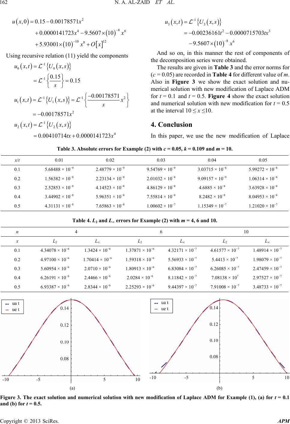
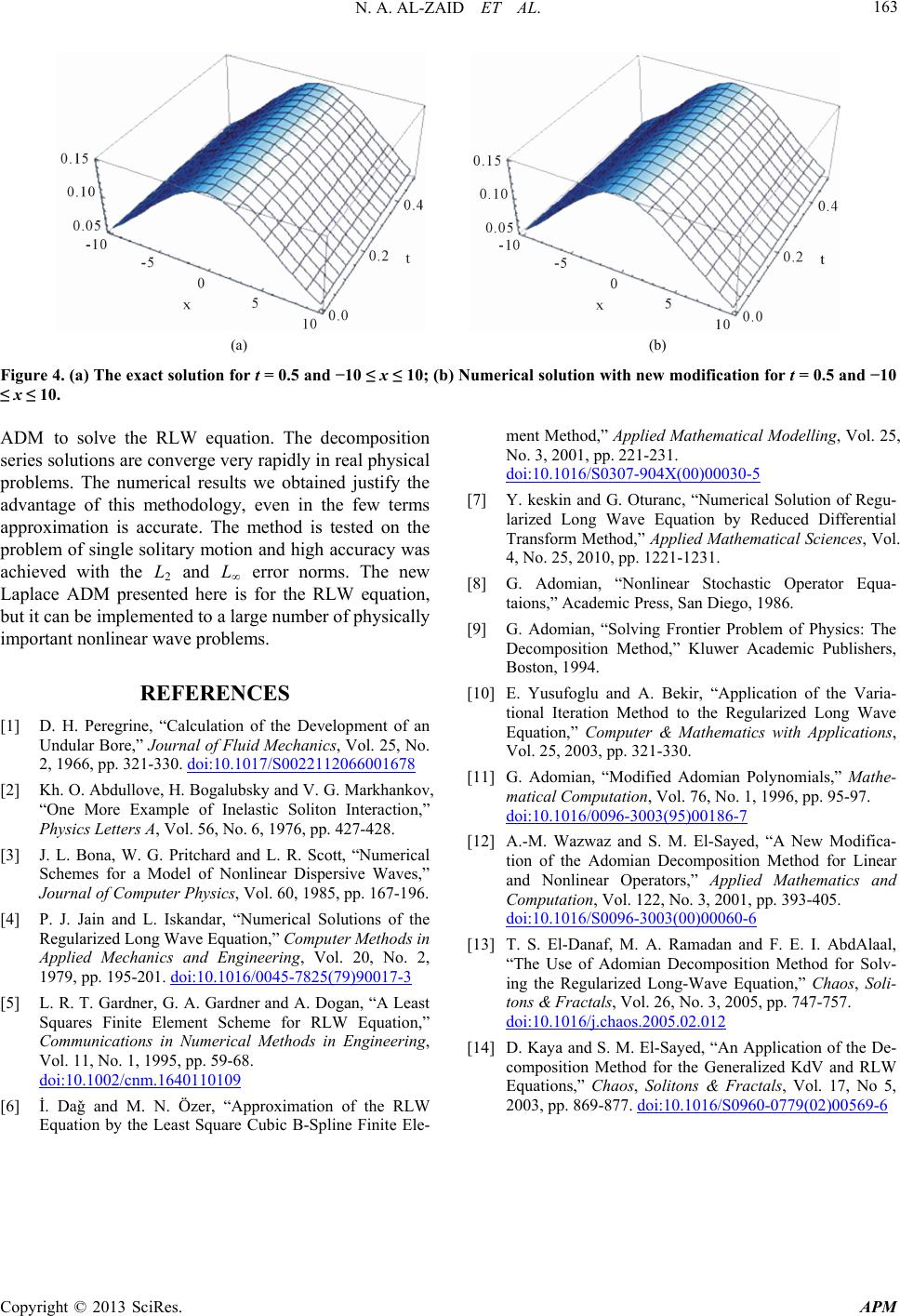
Figure 4. (a) The exact solution for t = 0.5 and −10 ≤ x ≤ 10; (b) Numerical solution with new modification for t = 0.5 and −10
≤ x ≤ 10.
ADM to solve the RLW equation. The decomposition
series solutions are converge very rapidly in real physical
problems. The numerical results we obtained justify the
advantage of this methodology, even in the few terms
approximation is accurate. The method is tested on the
problem of single solitary motion and high accuracy was
achieved with the L2 and L∞ error norms. The new
Laplace ADM presented here is for the RLW equation,
but it can be implemented to a large number of physically
important nonlinear wave problems.
REFERENCES
[1] D. H. Peregrine, “Calculation of the Development of an
Undular Bore,” Journal of Fluid Mechanics, Vol. 25, No.
2, 1966, pp. 321-330. doi:10.1017/S0022112066001678
[2] Kh. O. Abdullove, H. Bogalubsky and V. G. Markhankov,
“One More Example of Inelastic Soliton Interaction,”
Physics Letters A, Vol. 56, No. 6, 1976, pp. 427-428.
[3] J. L. Bona, W. G. Pritchard and L. R. Scott, “Numerical
Schemes for a Model of Nonlinear Dispersive Waves,”
Journal of Computer Physics, Vol. 60, 1985, pp. 167-196.
[4] P. J. Jain and L. Iskandar, “Numerical Solutions of the
Regularized Long Wave Equation,” Computer Methods in
Applied Mechanics and Engineering, Vol. 20, No. 2,
1979, pp. 195-201. doi:10.1016/0045-7825(79)90017-3
[5] L. R. T. Gardner, G. A. Gardner and A. Dogan, “A Least
Squares Finite Element Scheme for RLW Equation,”
Communications in Numerical Methods in Engineering,
Vol. 11, No. 1, 1995, pp. 59-68.
doi:10.1002/cnm.1640110109
[6] İ. Daǧ and M. N. Özer, “Approximation of the RLW
Equation by the Least Square Cubic B-Spline Finite Ele-
ment Method,” Applied Mathematical Modelling, Vol. 25,
No. 3, 2001, pp. 221-231.
doi:10.1016/S0307-904X(00)00030-5
[7] Y. keskin and G. Oturanc, “Numerical Solution of Regu-
larized Long Wave Equation by Reduced Differential
Transform Method,” Applied Mathematical Sciences, Vol.
4, No. 25, 2010, pp. 1221-1231.
[8] G. Adomian, “Nonlinear Stochastic Operator Equa-
taions,” Academic Press, San Diego, 1986.
[9] G. Adomian, “Solving Frontier Problem of Physics: The
Decomposition Method,” Kluwer Academic Publishers,
Boston, 1994.
[10] E. Yusufoglu and A. Bekir, “Application of the Varia-
tional Iteration Method to the Regularized Long Wave
Equation,” Computer & Mathematics with Applications,
Vol. 25, 2003, pp. 321-330.
[11] G. Adomian, “Modified Adomian Polynomials,” Mathe-
matical Computation, Vol. 76, No. 1, 1996, pp. 95-97.
doi:10.1016/0096-3003(95)00186-7
[12] A.-M. Wazwaz and S. M. El-Sayed, “A New Modifica-
tion of the Adomian Decomposition Method for Linear
and Nonlinear Operators,” Applied Mathematics and
Computation, Vol. 122, No. 3, 2001, pp. 393-405.
doi:10.1016/S0096-3003(00)00060-6
[13] T. S. El-Danaf, M. A. Ramadan and F. E. I. AbdAlaal,
“The Use of Adomian Decomposition Method for Solv-
ing the Regularized Long-Wave Equation,” Chaos, Soli-
tons & Fractals, Vol. 26, No. 3, 2005, pp. 747-757.
doi:10.1016/j.chaos.2005.02.012
[14] D. Kaya and S. M. El-Sayed, “An Application of the De-
composition Method for the Generalized KdV and RLW
Equations,” Chaos, Solitons & Fractals, Vol. 17, No 5,
2003, pp. 869-877. doi:10.1016/S0960-0779(02)00569-6