Computational Water, Energy, and Environmental Engineering, 2013, 2, 1-8
http://dx.doi.org/10.4236/cweee.2013.21001 Published Online January 2013 (http://www.scirp.org/journal/cweee)
Voltage Stability Constrained Optimal Power
Flow Using NSGA-II
Sandeep Panuganti1, Preetha Roselyn John1, Durairaj Devraj2, Subhransu Sekhar Dash1
1Department of Electrical and Electronics Engineering, Sri RamaswamyMemorial, Chennai, India
2DEAN (Research), Kalasalingam University, Krishnankoil, India
Received November 30, 2012; revised December 30, 2012; accepted January 8, 2013
ABSTRACT
Voltage stability has become an important issue in planning and operation of many power systems. This work includes
multi-objective evolutionary algorithm techniques such as Genetic Algorithm (GA) and Non-dominated Sorting Genetic
Algorithm II (NSGA-II) approach for solving Voltage Stability Constrained-Optimal Power Flow (VSC-OPF). Base
case generator power output, voltage magnitude of generator buses are taken as the control variables and maximum
L-index of load buses is used to specify the voltage stability level of the system. Multi-Objective OPF, formulated as a
multi-objective mixed integer nonlinear optimization problem, minimizes fuel cost and minimizes emission of gases, as
well as improvement of voltage profile in the system. NSGA-II based OPF—case 1—Two objective-Min Fuel cost and
Voltage stability index; case 2—Three objective—Min Fuel cost, Min Emission cost and Voltage stability index. The
above method is tested on standard IEEE 30-bus test system and simulation results are done for base case and the two
severe contingency cases and also on loaded conditions.
Keywords: Voltage Stability; Optimal Power Flow; Multi Objective Evolutionary Algorithms
1. Introduction
GA, invented by Holland in the early 1970s, is a stochas-
tic global search method that mimics the metaphor of
natural biological evaluation.Genetic Algorithms (GA) [1]
operates on a population of candidate solutions encoded
to finite bit string called chromosome. In order to obtain
optimality, each chromosome exchanges the information
using operators borrowed from natural genetic to produce
the better solution. The combined Economic-Emission
multiobjective problem seeks to simultaneously mini-
mize both fuel costand the emissions produced by power
plants. Environmental concerns on the effect of SO2 and
NOX emissions producedby the fossil-fueled power
plants led to the inclusion ofminimization of emissions as
an objective in the OPF formulation.
1.1. Voltage Stability
Voltage instability stems from the attempt of load dy-
namics to restore power consumption beyond the capa-
bility of the combined transmission and generation. Vol-
tage stability constrained OPF—Voltage stability indica-
tor is incorporated in the OPF formulation through the
L-index value. The voltage stability index is an appropri-
ate measure of the closeness of the system to voltage
collapse. NSGA-II is a popular non-domination based
genetic algorithm for multi-objective optimization which
has a better sorting algorithm and incorporates elitism
and no sharing parameter needed to be chosen as com-
pared to the original NSGA. Emission cost of generators
also play a vital role and is thus formulated in the mini-
mization OPF problem. Since OPF was introduced in
1968, several methods have been employed to solve this
problem, e.g. Gradient base, Linear programming me-
thod and Quadratic programming. However all of these
methods suffer from three main problems. Firstly, they
may not be able to provide optimal solution and usually
getting stuck at local optima [2]. Secondly, all these me-
thods are based on assumption of continuity and differen-
tiability of objective function which is not actually al-
lowed in a practical system.
1.2. VSC-OPF
The Contingencies such as unexpected line outages in a
stressed system may often result in voltage instability,
which may lead to voltage collapse. After a voltage col-
lapse, the system becomes dismantled owing to the
widespread operation of protective devices. Studies have
been performed to predict the voltage instability with
both static and dynamic approaches.
In this paper three different cases along with the sys-
tem loaded conditions are considered. In the first case
C
opyright © 2013 SciRes. CWEEE

S. PANUGANTI ET AL.
2
base case OPF as a single objective optimization problem
is solved using GA [3]. In the second case VSC-OPF
problem is formulated in MOGA with minimization of
fuel cost and L-index value. In the third case economic
emission of gases along with VSC-OPF problem is con-
sidered as a multi-objective problem and L-index is
solved using the NSGA-II approach in an IEEE 30 bus
system. NSGA [4] is a popular non-domination based
genetic algorithm for multi-objective optimization. It is a
very effective algorithm but has been generally criticized
for its computational complexity, lack of elitism and for
choosing the optimal parameter value for sharing pa-
rameter σ share. A modified version, NSGA-II [5] was
developed, which has a better sorting algorithm, incur-
porates elitism and no sharing parameter needs to be
chosen a priori.
2. Voltage Stability Index
The voltage stability analysis involves determination of an
index known as voltage collapse proximity indicator. This
index is an approximate measure of the closeness of the
system to voltage collapse. There are various methods of
determining the voltage collapse proximity indicator. One
such method is the L-index method proposed in Kessel
and Glavitsch. It is based on load flow analysis. Its value
ranges from 0 (no load condition) to 1 (voltage collapse).
The bus with the highest L-index value will be the most
vulnerable bus in the system. The technique is incorpo-
rated from [6]. The L-index calculation for a power sys-
tem is briefly discussed below.
Consider an N-bus system in which there are Ng gen-
erators. The relationship between voltage and current can
be expressed by the following expression:
·
busbus bus
I
YV (1)
By segregating the load buses (PQ) from generator
buses (PV), Equation (1) can write as
GG GL G
LG LL
G
L
L
YY
I
V
YY
I
V
  

 
  
(2)
where IG, IL and VG, VL represent currents and voltages at
the generator buses and load buses.
Rearranging the above equation we get:
LLLLGL
GGLGGG
VZFI
I
KYV
 

 
 
(3)
where:
 
1
L
GLLLG
F
YY


The L-index of the jth node is given by the expression:

1
1g
Ni
j
JIji ij
i
j
V
LF
V



 
 (4)
where:
Vi Voltage magnitude of ith generator
Vj Voltage magnitude of jth generator
θji Phase angle of the term Fji
δi Voltage phase angle of ith generator unit
δj Voltage phase angle of jth generator unit
Ng Number of generating units.
VL, I
L: Voltages and Currents for PQ buses; VG, IG: Voltages and Currents
for PV buses; Where, ZLL, FLG, KGL, YGG: sub matrices generated from Ybus
partial inversion.
Lj: L-index voltage stability indicator for bus k.
The values of Fji are obtained from the matrix FLG. The
L-indices for a given load condition are computed for all
the load buses and the maximum of the L-indices (Lmax)
gives the proximity of the system to voltage collapse.
The L-index has the advantage of indicating voltage in-
stability proximity of the current operating point without
calculation of the information about the maximum load-
ing point.
3. Problem Formulation
In general, the OPF problem is formulated as an optimi-
sation problem in which a specific objective function is
minimised while satisfying a number of equality and
inequality constraints[7]. The objectives of the OPF pro-
blem considered here are minimisation of fuel cost in the
normal state and the minimisation of the voltage stability
index Lmax in the emergency state. Power flow equations
are the equality constraints of the problem, while the
inequality constraints include the limits on real and reac-
tive power generation and bus voltage magnitude as fol-
lows.

1
1
Minimise
G
N
iGi iGi i
i
F
aP bP c


 (5)
max.
2
Minimise
F
L (6)

31
Minimise G
N
iGi iGii
i
F
dP ePg



D
(7)
min. max.
InequalityconstraintsGiGi Gi Gi PPP (8)
min. max.
iii
VVV (9)
min. max.
GiGi Gi
QQQ (10)
Equality Constraints G PP (11)
where:
N the number of total buses
NG the number of generator buses
NL the number of load buses
Nb the number of transmission lines
Pi,Qi real and reactive power injected at bus i
i
V Voltage magnitude at bus i

S. PANUGANTI ET AL. 3
The equality constraints given by the above equations
are satisfied by running the power flow program. The
active power generation (Pgi) (except the generator at the
slack bus) and generator terminal bus voltages (Vgi) are
the optimization variables and they are self-restricted by
the optimization algorithm.
4. Non-Dominated Sorting Genetic
Algorithm II (NSGA-II)
NSGA introduced by Srinivas and Deb [8], implements
the idea of a selection method based on classes of domi-
nance of all solutions. This algorithm identifies non-
dominated solutions in the population, at each generation,
to form non-dominated fronts, based on the concept of
non-dominance of Pareto. After this, the usual selection,
crossover, and mutation operators are performed.
However, there are some disadvantages in NSGA. It
has been generally criticized for its computational com-
plexity, lack of elitism and for choosing the optimal pa-
rameter value for sharing parameter σshare. A modified
version, NSGA-II was developed, which has a better
sorting algorithm, incorporates elitism and no sharing
parameter needs to be chosen a priori [9]. In this algo-
rithm, the population is initialized as random, and the
number of population is N. Once the population in ini-
tialized the population is sorted based on non-domina-
tion into each front. The first front being completely
non-dominant set in the current population and the sec-
ond front being dominated by the individuals in the first
front only and the front goes so on. Each Individual in
the each front are assigned rank values or based on front
in which they belong to. Then, crowding distance is cal-
culated for each individual. The crowding distance is a
measure of how close an individual is to its neighbours.
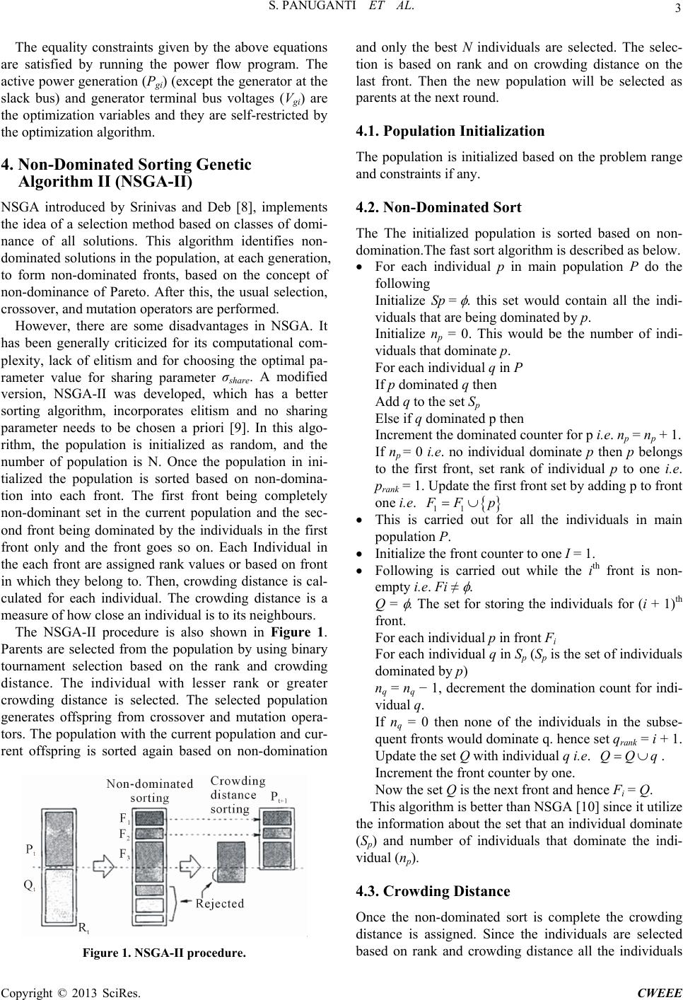
The NSGA-II procedure is also shown in Figure 1.
Parents are selected from the population by using binary
tournament selection based on the rank and crowding
distance. The individual with lesser rank or greater
crowding distance is selected. The selected population
generates offspring from crossover and mutation opera-
tors. The population with the current population and cur-
rent offspring is sorted again based on non-domination
Figure 1. NSGA-II procedure.
and only the best N individuals are selected. The selec-
tion is based on rank and on crowding distance on the
last front. Then the new population will be selected as
parents at the next round.
4.1. Population Initialization
The population is initialized based on the problem range
and constraints if any.
4.2. Non-Dominated Sort
The The initialized population is sorted based on non-
domination.The fast sort algorithm is described as below.
 For each individual p in main population P do the
following
Initialize Sp =
 . this set would contain all the indi-
viduals that are being dominated by p.
Initialize np = 0. This would be the number of indi-
viduals that dominate p.
For each individual q in P
If p dominated q then
Add q to the set Sp
Else if q dominated p then
Increment the dominated counter for p i.e. np = np + 1.
If np = 0 i.e. no individual dominate p then p belongs
to the first front, set rank of individual p to one i.e.
prank = 1. Update the first front set by adding p to front
one i.e.


11
FpF
 This is carried out for all the individuals in main
population P.
 Initialize the front counter to one I = 1.
 Following is carried out while the ith front is non-
empty i.e. Fi ≠
 .
Q =  . The set for storing the individuals for (i + 1)th
front.
For each individual p in front Fi
For each individual q in Sp (Sp is the set of individuals
dominated by p)
nq = nq − 1, decrement the domination count for indi-
vidual q.
If nq = 0 then none of the individuals in the subse-
quent fronts would dominate q. hence set qrank = i + 1.
Update the set Q with individual q i.e. . QQq
Increment the front counter by one.
Now the set Q is the next front and hence Fi = Q.
This algorithm is better than NSGA [10] since it utilize
the information about the set that an individual dominate
(Sp) and number of individuals that dominate the indi-
vidual (np).
4.3. Crowding Distance
Once the non-dominated sort is complete the crowding
distance is assigned. Since the individuals are selected
based on rank and crowding distance all the individuals

S. PANUGANTI ET AL.
4
in the population are assigned a crowding distance value.
Crowding distance is assigned front wise and comparing
the crowding distance between two individuals in differ-
ent front is meaningless. The crowing distance is calcu-
lated as below
 For each front Fi, n is the number of individuals.
 Initialize the distance to be zero for all the individuals
i.e. Fi(dj) = 0, where j corresponds to the jth individ-
ual in front Fi.
 For each objective function m.
 Sort the individuals in front Fi based on objective m
i.e., i = sort (Fi, m).
 Assign infinite distance to boundary values for each
individual in Fi i.e.

1
Id

 and

IDn

.
 For k = 2 to (n − 1)




max min
11
.
kk
mm
I
kmIkm
Id Idff
 
  (12)
 I(k)·m is the value of the mth objective function of the
kth individual in I.
The basic idea behind the crowing distance is finding
the euclidian distance between each individual in a front
based on their m objectives in the m dimensional hyper
space. The individuals in the boundary are always se-
lected since they have infinite distance assignment.
4.4. Selection
Once the individuals are sorted based on non-domination
and with crowding distance assigned, the selection is
carried out using a crowded-comparison-operator (an).
The comparison is carried out as below based on
1) Non-domination rank prank i.e. individuals in front Fi
will have their rank as prank = i.
2) Crowding distance Fi(dj)
 p an q if
 prank < qrank
 or if p and q belong to the same front Fi then Fi(dp) >
Fi(dq) i.e. the crowing distance should be more.
The individuals are selected by using a binarytourna-
ment selection with crowed-comparison-operator.
4.5. Genetic Operators
NSGA-II use Simulated Binary Crossover (SBX)
[10,11] and polynomial mutation [10,12].
4.5.1 Simulated Binary Crossover
The Simulated binary crossover simulates the binary
crossover observed in nature and is give as below.


1,1, 2,
2,1, 2,
111
2
111
2
kkkk
kkkk
Cp
Cp




 

where Ci,k is the ith child with kth component, Pi,k is the-
selected parent and βk (≥) is a sample from a random
number generated having the density
 


2
11,if0 1
2
11
1,if 1
2
c
c
c
c
p
p


 
 









 



(14)
This distribution can be obtained from a uniformly
sampled random number u between (0, 1). ηc is the dis-
tribution index for crossover. That is
 



1
1
1
1
2
121
uu
uu















(15)
4.5.2. Polynomial Mutation

ul
kk kk
cp pp
k

  (16)
where ck is the child and pk is the parent with being
the upper boundon the parent component, is the
lower bound and k
u
k
p
l
k
p

is small variation which is calcu-
lated from a polynomial distribution by using


1
1
1
1
21,if0.5
121,if 0.5
m
m
kk k
kkk
rr
rr












 
 
(17)
rk is an uniformly sampled random number between (0,1)
and ηm is mutation distribution index.
4.6. Recombination and Selection
The offspring population is combined with the current
generation population and selection is performed to set
the individuals of the next generation. Since all the pre-
vious and current best individuals are added in the popu-
lation, elitism is ensured. Population is now sorted based
on non-domination. The new generation is filled by each
front subsequently until the population size exceeds the
current population size. If by adding all the individuals in
front Fj the population exceeds N then individuals in
front Fj are selected based on their crowding distance in
the descending order until the population size is N. And
hence the process repeats to generate the subsequent
generations.
5. Best compromised Solution
k
k
p
p







 
 


(13)
Upon having the pareto-optimal set of non-dominated
solution, the proposed approach [8] presents a best com-
promise solution tothe decision maker. Due to the impre-
cise nature of the decision maker’s judgement, the ith
objective function Ji is represented bya membership
function defined as

S. PANUGANTI ET AL. 5

min
max
min max
max min
max
1,
,
0,
ii
ii
ii
ii
ii
JJ
JJ
ii
J
JJJ
JJ
JJ












 (18)
where max
i
J
and min
i
J
are the maximum and minimum
values of the ith objective function among all non-domi-
nated solutions.
For each non-dominated solution k, the normalized
membership function
K
D

is calculated as



1
5
11
K
KK
i
I
KK
i
k
D
i
J
J






 (19)
6. Simulation Results
The proposed NSGA-II approach has been applied to
solve the VSC-OPF problem in an IEEE 30-bus test sys-
tem. The system has six generator buses, 24 load buses
and 41 transmission lines.The generator cost coefficients
and the transmission line parameters are taken from [12].
Three different cases were considered for simulation, one
without considering the voltage stability i.e, to solve the
VSC-OPF problem using MOGA and the second one is
solved having economic emission of gases including
VSC-OPF in NSGA-II.These simulations were imple-
mented using the MATLAB program. The results of
these simulations are presented, Figure 2.
In this case the two objectives are minimization of fuel
cost and minimization of L-index using multi-objective
Genetic Algorithm. The results of VSC-OPF using
MOGA is shown in Table 1.
6.1. (Case 1): VSC-OPF Using NSGA-II
The voltage stability index (L-index) was included as the
second objective function of the OPF problem along with
the base fuel cost. The NSGA-II based algorithm was
applied to solve this VSC-OPF problem. The optimal
control variable setting obtained in this case is presented
in Table 2 alongwith the L-index value. In Figure 4
shows the pareto optimal front of generation cost and
L-index is shown and the Table 2 shows the line outage
27 - 28 along with line outage 27 - 30 is shown in Table
3.The solution is a set of non-dominated solutions. The
comparison of the results obtained in NSGA-II and three
objective is shown in Table 5. From this table it is clear
that the performance of NSGA-II is better than MOGA in
VSC-OPF problem.
Contingency analysis was conducted on the system
with 125% loaded condition by simulating the single line
outages and in each case the maximum L-index value
was evaluated. From the contingency analysis it was
found that line outage 28 - 27 is the most severe one
Table 1. NSGA-II base case.
Control
Va ria bl es
Min F1
(Fuel cost)
Min F2
(L-index)
Best
compromised sol.
P1 169.6545 140.9243 168.6642
P2 50.0000 80.0000 50.4760
P5 23.9893 42.9811 24.1108
P8 22.0474 18.9395 22.1680
P11 13.2559 17.0000 13.4598
P13 14.8000 20.4000 14.8000
V1 1.0000 1.0000 1.0000
V2 1.0000 1.0040 1.0000
V5 0.9826 1.0000 0.9991
V8 0.9884 1.0000 0.9891
V11 0.9899 0.9903 0.9918
V13 0.9874 0.9888 0.9933
Fuel cost, F1 807.1765 872.7911 807.9227
L-index , F2 0.1101 0.1075 0.1095
800 810820 830 840 850 860870 880
0. 107
0.1075
0. 108
0.1085
0. 109
0.1095
0. 11
0.1105
0. 111
0.1115
0. 112
L-INDEX
FUEL COST
Figure 2. NSGA-II base case.
from the voltage security point of view during this con-
tingency state.
Table 6 gives the fuel cost, Lmax and minimum voltage
value of the contingency constrained VSC-OPF using
NSGA-II. This reduction in Lmax is obtained at the ex-
pense of increased fuel cost. Figure 5 shows the pareto
optimal front of contingency constrained VSC-OPF.
The line outage for 27 - 30 as shown in Figure 4, in
Tables 4, 5 and is also performed along with the same
loaded condition as in line outage 27 - 28 as shown in
Figure 3 and results are tabulated. The reduction in
L-max is obtained at the extent of increased fuel cost.

S. PANUGANTI ET AL.
6
Table 2. NSGA II—Line outage 27 - 28.
Control
Va ria bl es
Min F1
(Fuel cost)
Min F2
(L-index)
Best
compromised sol.
P1 174.9058 112.3927 149.0853
P2 50.000 80.0000 61.6056
P5 22.0000 41.7412 27.7161
P8 22.500 22.4915 19.6752
P11 12.8957 16.1521 16.8888
P13 14.8000 20.3995 20.4000
V1 1.000 1.0000 1.0000
V2 1.000 0.9901 0.9988
V5 0.9874 0.9874 0.9856
V8 0.9917 1.0040 0.9911
V11 0.9903 0.9902 1.0000
V13 0.9866 0.9866 0.9859
Fuel cost, F1 814.0790 876.6776 814.2402
L-index, F2 0.2905 0.2877 0.2895
Table 3. NSGA-2—Line outage 27 - 30.
Control
Va ria bl es
Min F1
(Fuel cost)
Min F2
(L-index)
Best
compromised sol.
P1 173.2358 107.6728 147.3212
P2 50.0000 80.0000 55.1566
P5 22.2229 42.9728 30.5305
P8 19.2142 22.5000 22.3421
P11 15.1615 17.0000 17.0000
P13 14.8000 20.4000 20.2354
V1 1.0000 1.0000 1.0000
V2 1.0000 0.9990 0.9984
V5 0.9793 0.9876 0.9844
V8 0.9866 1.0020 1.0020
V11 0.9875 0.9930 0.9914
V13 0.9835 0.9902 0.9886
Fuel cost, F1 810.0262 876.3660 812.5044
L-index , F2 0.1989 0.1953 0.1964
6.2. (Case 2): Economic Emission Based
VSC-OPF Using NSGA-II
The economic emission of the gases are included as the
third objective along with the voltage stability index and
810 820 830 840850 860 870880890
0. 28 8
0. 28 9
0. 29
0. 29 1
0. 29 2
0. 29 3
0. 29 4
0. 29 5
0. 29 6
0. 29 7
L-INDEX
FUEL COST
Figure 3. NSGA-II—Line outage 27 - 28.
Figure 4. NSGA-2—Line outage 27 - 30.
Figure 5. NSGA 2—3 Objective base case.
base fuel cost. The NSGA-II based algorithm was applied
to solve this VSC-OPF problem. The optimal control
variable settings are similar to that of the two objective
case. In Figure 5 shows the pareto optimal front of gen-
eration cost, L-index and economic emission dispatch of
gases for base case and in Figures 6, 7 the line outage 27
- 28 and line outage 27 - 30 are also included.

S. PANUGANTI ET AL. 7
Table 4. NSGA-II—3 objective line outage 27 - 28.
Control
Va ria bl es
Min F1
(Fuel cost)
Min F2
(L-index)
Min
Emission, F3
Best
compromised sol.
P1 160.3011 165.1097169.5373 162.3011
P2 65.7505 60.3991 57.8956 66.7505
P5 23.3074 25.8083 22.000 24.3172
P8 16.6748 14.5257 15.4874 16.6738
P11 12.8745 13.0869 14.3629 12.6730
P13 14.8000 14.9005 14.8981 14.8230
V1 1.000 1.000 1.000 1.000
V2 1.000 1.000 1.000 1.000
V5 0.9999 1.000 0.9999 0.9999
V8 0.9999 1.000 0.9999 0.9899
V11 0.9999 1.000 1.000 0.9994
V13 0.9999 0.9999 1.000 0.9999
Fuel cost,
F1 807.0019 853.6211856.5133 809.0019
L-index,
F2 0.1102 0.1077 0.1083 0.1099
Emission,
F3 1424.5 1324.0 1316.2 1386.5
Table 5. NSGA-2—Line outage 27 - 30.
Control
Va ria bl es
Min F1
(Fuel cost)
Min F2
(L-index)
Min
Emission, F3
Best
compromised sol.
P1 170.8424 167.0531 145.6723 168.5707
P2 50.000 57.9636 69.0360 57.4857
P5 23.1042 23.8583 23.2324 23.0908
P8 21.3731 16.0485 20.4102 15.9655
P11 14.2896 12.6677 15.5218 12.8070
P13 14.8000 16.8955 19.3528 16.6933
V1 1.000 1.000 1.000 1.000
V2 1.000 1.000 1.000 1.000
V5 0.9989 1.000 0.9999 0.9999
V8 0.9883 0.9991 0.9999 1.000
V11 0.9914 1.000 0.9999 0.9999
V13 0.9925 0.9999 1.000 0.9999
Fuel cost,
F1 809.9571 874.2141 844.7509 810.5175
L-index ,
F2 0.1978 0.1944 0.1961 0.1954
Emission ,
F3 1413.7 1305.8 1325.7 1316.8
Figure 6. NSGA-2—Line outage 27 - 28.
Figure 7. NSGA-2—Line outage 27 - 30.
7. Conclusion
In this paper, the various aspects of single-objective op-
timal power flow and multi-objective voltage stability
constrained optimal power flow are studied. An efficient
and diversified approach using NSGA-II algorithm is
identified to solve the above multi-objective optimization
problems. Several case studies have been employed
separately for single & multi-objective optimization
problem. Firstly, the results are obtained for single ob-
jective OPF and contingency constrained VSC-OPF us-
ing genetic algorithm for the optimization of Fuel cost
which are then compared with the power flow results of
other papers. The multi-objective VSC-OPF problem is
formulated using NSGA-II algorithm. The proposed al-
gorithm occupies less memory space and takes CPU time
than conventional GA approach. Simulation results of the
IEEE 30-bus system have been presented to illustrate the
effectiveness of the proposed approach to solve the
VSC-OPF problem. This simulation results were carried
out using NSGA-II and are found that voltage stability is

S. PANUGANTI ET AL.
8
improved in NSGA-II than multi-objective GA of the
proposed algorithm than the other approaches.
REFERENCES
[1] N. Srinivas and K. Deb, “Multi-Objective Optimization
Using Nondominated Sorting Ingenetic Algorithms,”
Technical Report, Department of Mechanical Engineering,
Indian Institute of Technology, Kanpur, 1993.
[2] N. Srinivas and K. Deb, “Multi-Objective Optimization
Using Nondominated Sortingin Genetic Algorithms,” Evo-
lutionary Computation, Vol. 2, No. 3, 1994, pp. 221-248.
doi:10.1162/evco.1994.2.3.221
[3] A. J. Wood and B. F. Wollenberg, “Power Generation Ope-
ration and Control,” John Wiley & Sons, Inc., New York,
1996.
[4] M. S. Kumari, “Enhanced Genetic Algorithm Based Com-
putation Technique for Multi-Objective, Optimal Power
Flow Solution,” Electrical Power and Energy Systems, Vol.
32, No. 6, 2010, pp. 736-742.
[5] K. O. Alawode, A. M. Jubril and O. A. Komolafe, “Multi-
Objective Optimal Power Flow Using Hybrid Evolutiona-
ry Algorithm,” International Journal of Electrical Power &
Energy Systems Engin, Vol. 3, No. 3, 2010, p. 196.
[6] D. Devaraj and J. P. Roselyn, “Improved Genetic Algo-
rithm for Voltage Security Constrained Optimal Power
Flow Problem,” International Journal of Energy Tech-
nology and Policy, Vol. 5, No. 4, 2007, pp. 475-488.
doi:10.1504/IJETP.2007.014888
[7] H. Sadat, “Power Systems Analysis,” McGraw Hill Pub-
lication, New Delhi, 1997.
[8] O. Alsac, and B. Scott, “Optimal Load Flow with Steady
State Security,” IEEE Transactions on Power Systems,
Vol. PAS-93, No. 3, 1974, pp.745-751.
doi:10.1109/TPAS.1974.293972
[9] H. W. Dommel and W. F. Tinney, “Optimal Power Flow
Solutions,” IEEE Transactions on Power Apparatusand Sys-
tems , Vol. PAS-87, No. 10, 1968, pp. 1866-1876.
[10] S. Dhanalakshmi, S. Kannan, K. Mahadevan and S. Bas-
kar, “Application of Modified NSGA-II Algorithm to Com-
bined Economicand Emission Dispatch Problem,” Inter-
national Journal of Electrical Power & Energy Systems,
Vol. 33, No. 4, 2011, pp. 992-1002.
[11] R. He, G. A. Taylor and Y. H. Song, “Multi-Objective
Optimal Reactive Power Flow including Voltage Security
and Demand Profile Classification,” International Jour-
nal of Electrical Power & Energy Systems, Vol. 30, No. 5,
2008, pp. 327-336.
[12] K. O. Alawode, A. M. Jubril and O. A. Komolafe, “Multi-
Objective Optimal Reactive Power Flow Using Elitist
Nondominated Sorting Genetic Algorithm: Comparison
and Improvement,” Journal of Electrical Engineering &
Technology, Vol. 5, No. 1, 2010, pp. 70-78.