J. Service Science & Management, 2010, 3, 309-335
doi:10.4236/jssm.2010.33038 Published Online September 2010 (http://www.SciRP.org/journal/jssm)
309
A Statistical Analysis to Predict Financial Distress
Nicolas Emanuel Monti, Roberto Mariano Garcia
Department of Industrial Engineering, Instituto Tecnológico de Buenos Aires (ITBA), Buenos Aires, Argentina.
Received June11th, 2010; revised July 17th, 2010; accepted August 20th, 2010.
ABSTRACT
The aim of this study is to apply the statistical inference to identify if a firm is likely to become financially distressed in
the short term. To do this, we decided to collect data from the firms’ financial statements. The analyses performed were
based on a group of 45 financial ratios observed from a sample of 86 firms operating in Argentina. First, we used the
principal component analysis to turn the information in the 45 original ratios into two new global variables named as
∆Risk and ∆Return. In this way, we can easily represent and compare in a graph the firms’ risk and return variations.
By the computation of these new variables it is possible to quickly financially categorize a certain firm based on the risk
the company has with regard to the nature of its business and the risk involved in the amount of debt it has taken in
comparison to the profits that were generated during the last two fiscal years. Second, we performed a logistic regres-
sion analysis to estimate the probability that a firm becomes financially distressed in the short term. The model finally
selected managed to successfully identify 85% of the companies from the sample and it explains 65% of the total sample
variability. The model is represented by the following variables: 1) Current Debt Ratio, 2) Total Cost of Debt, 3) Oper-
ating Profit Margin, and 4) ∆ROE. The outcomes from this study are two tools that were developed based on the statis-
tical inference from which we can quickly asses the financial status of a firm based on its risks and return’s variation as
well as to estimate the probability that a firm becomes financially distressed in the short term. There are different ways
of taking these tools into practice such as: 1) to control and follow up the financial performance of a company, 2) to
support the decision of lending money to a company, 3) to support the decision of investing money or the decision of
merging with a company, 4) to support market analysis from a financial perspective, and 5) to support actions or deci-
sions related to the financial assessment of a company that declares itself to be financially distressed.
Keywords: Financial Distress, Financial Risk, Principal Component Analysis, Logistic Regression Analysis
1. Introduction
The objective of this study is to identify those companies
that have financial problems based on the information
contained on their financial statements. With this regard,
it is considered that a company has financial problems
when it has a high probability of becoming financially
distressed in the short term. To do this, we applied the
statistical inference to a group of 45 financial ratios ob-
served from a sample of 86 firms operating in Argentina.
In previous similar studies, as for example those pro-
posed by Guzmán [1], Heine [2], De la Torre Martínez [3]
or Kahl [4], it was suggested as an objective to find that
financial ratio that could better identify a company with
financial problems or to find that statistical model that
could better predict if a company is financially distressed
based on the discriminant analysis. Although all these
approaches might be efficient to identify which aspects
of a company we should focus on when trying to asses its
financial situation, their statistical outcomes would typi-
cally not be able to provide a good overview of the firms’
overall performance as they are based on just a few vari-
ables. This means that with the current statistical models
it would be possible to recognize when a company is
financially unhealthy but it would be difficult to identify
under what circumstances a firm reached that status or
even to compare how critical its financial situation is in
comparison to other business units or companies within
the same industry. Moreover, most of the statistical stud-
ies in the current literature do not take into consideration
the variation of the firms’ financial ratios through the last
fiscal periods. Instead they provide a financial diagnosis
based on the most recent snapshot of the firms’ situation,
which might result in wrong decisions being made.
In an attempt to provide a financial study that can
cover the issues previously discussed, we decided to

A Statistical Analysis to Predict Financial Distress 310
combine two statistical analyses with the aim of devel-
oping a set of tools that will provide a comprehensive
and accurate financial diagnosis of a firm that can be
used to take decisions within different business scenarios
such as investments analysis, credits offering, and finan-
cial management, among others. In this way, we first
used the principal component analysis to turn all the data
initially collected into two new variables. With this
analysis we can obtain a financial overview of a certain
firm and we can represent and compare its financial
situation based on the risk the company has with regard
to the nature of its business and the risk involved in the
amount of debt it has taken in comparison to the profits
that were generated during the last two fiscal years. Sec-
ond, we used the logistics regression analysis to precisely
determine when a firm has financial problems and to
identify those ratios that have a higher influene on its
financial condition.
The rest of this paper is organized as follows. In Sec-
tion 2, we present the sample design by defining its size
and composition as well as the criteria used to collect all
the data from the firms’ financial statements. In Section 3,
we define the group of 45 financial ratios that were
computed for each company in the sample. In Section 4,
the principal component analysis is performed to turn the
information contained in the 45 original ratios into a
small group of 2 new variables named as ∆Risk and
∆Return. In Section 5, we developed different logistic
regression models to estimate the probability that a firm
becomes financially distressed in the short term. In Sec-
tion 6, the tools developed from the principal component
and the logistic regression analyses are applied to a new
sample. The objective in this case is to evaluate the joint
effectiveness of these tools to recognize those companies
with financial problems. Finally, the conclusions of the
present study together with its possible uses are described
in Section 7.
2. Sample Design
A very important aspect in this kind of statistical research
is the sample design from which the statistical models
will be developed. For example, if we consider a sample
of companies that belong to the construction sector then
the resulting statistical model can only be applied to
companies of that sector. Also, if the sample is composed
by 90% of companies that did not have any financial
problems and only 10% of companies that were finan-
cially distressed then the capacity of any resulting statis-
tical model to discriminate companies with financial
problems will not be significant. Because of these rea-
sons, below we comment all the criteria considered to
design the sample which will determine the scope of the
analysis.
The sample is composed by 86 firms that operate in
Argentina, from which 43 did not have any financial
problems (group 1) and the other 43 were financially dis-
tressed during the period under analysis (group 2). See
Appendix 1 for a complete sample description.
All the information considered in the present study
was obtained from the financial statements of each com-
pany. In the case of those companies that did not have
any financial problem, the financial statements were ob-
tained from the Bolsa de Comercio de Buenos Aires
(BCBA). For those companies that had financial prob-
lems, the financial statements were obtained from the
official reports made by the corresponding receivers that
are published by the Cámara Nacional de Apelaciones en
lo Comercial.
Different authors from statistical books consider valid
to collect at least information from 5 observations for
each variable that is included in the statistical model.
William Beaver [5] and Edward Altman [6] carried out
similar statistical analysis working with a sample of 120
and 60 companies, respectively. In both cases, significant
results were obtained and they both considered different
models with no more than 5 variables. Therefore, based
on these results and considering that in the present study
we will not develop any model with more than 5 vari-
ables, we can state that a sample of 86 firms is big
enough to carry out any statistical analysis.
With regard to the proportion of companies in the
sample with and without financial problems, it is not
strictly necessary to consider the same amount of obser-
vations for each of these groups. However, this is rec-
ommended to obtain a better representation of the mean
and the deviation of the variables observed in each group.
To better understand this issue, we can consider the ex-
treme case of a sample with 1 company that did not have
any financial problems and 99 companies that were fi-
nancially distressed. Based on this sample, when it comes
the moment to estimate the probability that a firm be-
comes financially distressed it is reasonable to think that
the corresponding model will have a clear tendency to
classify any company as if it is going to have financial
problems in the near future. This is because the sample,
while not being representative from the population, does
not “reveal” the different ways in which a company with-
out financial problems can be found. In other words, the
sample contains very little information about the behav-
ior of the variables observed in companies without finan-
cial problems, and therefore, it is more difficult for the
model to recognize companies from this group.
Another important aspect to consider is the period of
time from which the information in the financial state-
ments is collected, especially in the case of those compa-
nies that had financial problems. With this regard, the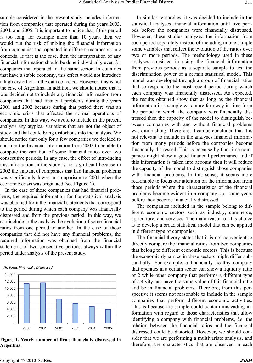

A Statistical Analysis to Predict Financial Distress 311
sample considered in the present study includes informa-
tion from companies that operated during the years 2003,
2004, and 2005. It is important to notice that if this period
is too long, for example more than 10 years, then we
would run the risk of mixing the financial information
from companies that operated in different macroeconomic
contexts. If that is the case, then the interpretation of any
financial information should be done individually even for
companies that operated in the same sector. In countries
that have a stable economy, this effect would not introduce
a high distortion in the data collected. However, this is not
the case of Argentina. In addition, we should notice that it
was decided not to include any financial information from
companies that had financial problems during the years
2001 and 2002 because during that period there was an
economic crisis that affected the normal operations of
companies. In this way, we avoid to include in the present
analysis any atypical variations that are not the object of
study and that could bring distortions into the analysis. We
should notice that only for a few companies we decided to
consider the financial information from 2002 to be able to
compute the variation of some financial ratios over two
consecutive periods. In any case, the effect of introducing
this information in the study is not significant because in
2002 the amount of companies that had financial problems
was significantly lower in comparison to 2001 when the
economic crisis was originated (see Figure 1).
In the case of those companies that had financial prob-
lems, the required information for the statistical analysis
was obtained from the financial statements that correspond
to the period during which each company was financially
distressed and from the previous period. In this way, we
can include in the analysis the evolution of some financial
ratios from one period to another. In the case of those
companies that did not have any financial problems, the
required information was obtained from the financial
statements of two consecutive periods, always within the
period under analysis of the present study.
0
2,000
4,000
6,000
8,000
10,000
12,000
14,000
2000 2001 2002 2003 2004 2005
Nr. Firms Financially Distressed
Figure 1. Yearly number of firms financially distressed in
Argentina.
In similar researches, it was decided to include in the
statistical analyses financial information until five peri-
ods before the companies were financially distressed.
However, these studies analyzed the information from
each period separately instead of including in one sample
some variables that reflect the evolution of the ratios over
two or more periods. The methodology used in these
analyses consisted in using the financial information
from previous periods as a separate sample to test the
discrimination power of a certain statistical model. This
model was developed through a group of financial ratios
that correspond to the most recent period during which
each company was financially distressed. As expected,
the results obtained show that as long as the financial
information in a sample was more far away in time from
the period in which the company was financially dis-
tressed then the capacity of the model to distinguish be-
tween companies with and without financial problems
was diminishing. Therefore, it can be concluded that it is
not relevant to include in the analyses financial informa-
tion from many periods before the companies become
financially distressed. This is because by that time com-
panies might show a good financial performance and if
this information is taken into account then it will reduce
the capacity of the model to distinguish those companies
with financial problems. In this sense, it seems more
reasonable to focus our attention on the information from
those periods where the characteristics of the financial
problems become evident in a company, i.e. some years
before they become financially distressed.
The companies included in the sample belong to dif-
ferent economic sectors such as industry, commerce,
agriculture, and services. The main reason of this choice
is to develop a broad statistical model that can be applied
in different type of companies.
The financial theory states that it is not convenient to
directly compare the financial ratios from two companies
that belong to different economic sectors. This is because
the economic dynamics in these sectors might differ sub-
stantially. For example, a financially healthy company
that operates in a certain sector can show a liquidity ratio
of 2 while other company that performs a different type
of activity can have the same value of this financial ratio
and be in financial problems. Therefore, from this per-
spective it seems not reasonable to include in the sample
companies that perform different economic activities.
This is because the sample could contain misleading in-
formation with regard to those characteristics that allow
identifying a company with financial problems, i.e. the
relation between the financial ratios and the financial
distressed could be distorted. However, we should con-
sider that we are performing a multivariate analysis, and
therefore, the characteristics that are observed in each

A Statistical Analysis to Predict Financial Distress 312
individual are compared in a simultaneous and global
way. In this way, it is more difficult that the particular
behavior of certain ratios in some economic sectors af-
fect the global profile of a company. Nevertheless, there
are two precautions that can be implemented in order to
diminish the effect that some characteristics inherit to
each economic sector have in the identification of com-
panies with financial problems. The first precaution con-
sists of including in both groups of the sample companies
from the same economic sectors. The second precaution
consists of having the same amount of companies from
each economic sector in both sample groups. Although
the second precaution was not implemented for all the
economic sectors because of the difficulties to find
available financial data, the sample was design to keep
the highest balance possible in both groups.
William Beaver [5] designed a paired sample based on
companies that operated in different economic sectors. In
that sample, for every company that had financial prob-
lems there was another financially healthy company from
the same economic sector, and whenever it was possible,
with the same size. With this regard, we should notice
that the size of a company was measured through its total
assets. In this way, Beaver performed a univariate statis-
tical analysis, i.e. that the financial ratios of each com-
pany were compared once at a time and that the distinc-
tion of those companies with financial problems was
made through a single ratio with a cut-off value.
In his research, Beaver suggested doing a paired
analysis with the objective of quantifying the effect that
the economic sectors and the size of the companies have
in the identification of those companies financially dis-
tressed. In this way, for each pair of companies from the
same economic sector and with similar sizes the differ-
ence of each financial ratio was computed. Afterwards,
these differences were evaluated to determine if there
was sufficient statistical evidence that allowed the identi-
fication of companies with financial problems. We should
notice that because each difference of the financial ratios
was determined based on companies from the same eco-
nomic sector and with similar sizes, the effects of these
factors in the sample were mitigated. In addition, it is
important to mention that these differences were only
computed to quantify the impact that the economic sec-
tors and the size of the companies have on the identifica-
tion of those companies with financial problems. How-
ever, to classify each firm in one of the two groups a
limit value from a single financial ratio was considered.
This limit value was computed through a direct com-
parison of the financial ratios, i.e. no differences between
the financial ratios were considered. The reason of this is
that it is not possible to get any conclusions from a single
individual through a paired analysis because always two
companies are compared at the same time.
Once the paired analysis is performed, the capacity of
each financial ratio to identify those companies with fi-
nancial problems can be compared to those capacities
that are obtained from a statistical analysis based on a
global comparison of the companies. With this regard,
one would expect these results to be similar as long as
the effect of the economic sectors and the size of the
companies were negligible. In fact, the findings from
Beaver’s research support this statement. Therefore,
everything seems to indicate that using a paired sample is
the best approach to mitigate the possible effects from
the economic sectors and the size of the companies.
However, we must take into account that the research
made by Beaver was based on a univariate statistical
analysis, and therefore, each financial ratio was com-
pared once at a time. This means that the effects of these
factors when multiple financial ratios are compared at the
same time were not evaluated. In this sense, we expect
that by simultaneously comparing multiple financial ra-
tios the effects of the economic sectors and the size of the
companies should also be mitigated. Therefore, we can
conclude that it is not strictly necessary to have a paired
sample to continue with our study although keeping a
certain balance in the sample can help to diminish the
undesired effects of the economic sectors and the size of
the companies.
Another precaution that has been considered in the
present study to facilitate the identification of companies
with financial problems in different economic sectors is
the incorporation of a variable that measures the per-
formance of a given company in comparison to the aver-
age performance of the sector. More details about the
variables considered can be found in the following sec-
tion.
Finally, another important aspect to be considered in
the sample design is the size of the companies. This as-
pect has already been mentioned when referring to Bea-
ver’s research. With this regard, the sample was designed
not to include companies with high assets value, i.e. all
the companies included in the statistical analysis have
assets lower than 500 [Million $AR]. The reason of this
is that there are just a few cases where big companies
suffered financial problems, and therefore, it is reason-
able to think that these firms belong to a different statis-
tical population. With this regard, Alexander Sydney [7]
suggests that there is theoretical evidence as well as em-
pirical facts that demonstrate that the return rate of a
company becomes more stable as the size of its assets
increases. This could imply that a firm with a high assets
value would have a lower risk of becoming financially
distressed in comparison to a middle size or small com-
pany even when they both show the same financial ratios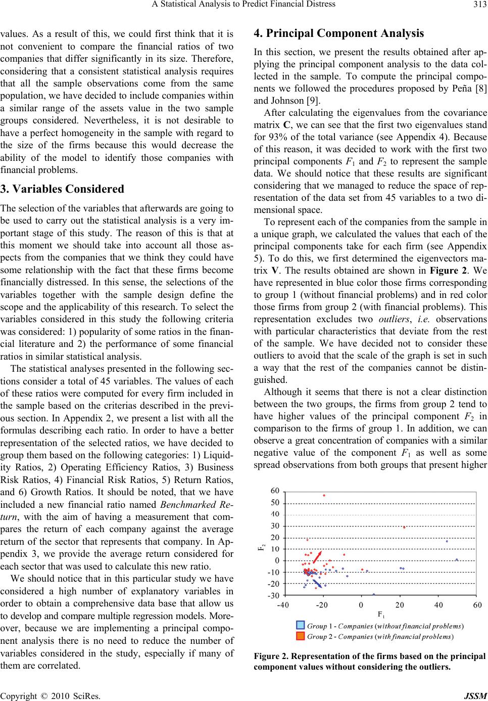

A Statistical Analysis to Predict Financial Distress 313
values. As a result of this, we could first think that it is
not convenient to compare the financial ratios of two
companies that differ significantly in its size. Therefore,
considering that a consistent statistical analysis requires
that all the sample observations come from the same
population, we have decided to include companies within
a similar range of the assets value in the two sample
groups considered. Nevertheless, it is not desirable to
have a perfect homogeneity in the sample with regard to
the size of the firms because this would decrease the
ability of the model to identify those companies with
financial problems.
3. Variables Considered
The selection of the variables that afterwards are going to
be used to carry out the statistical analysis is a very im-
portant stage of this study. The reason of this is that at
this moment we should take into account all those as-
pects from the companies that we think they could have
some relationship with the fact that these firms become
financially distressed. In this sense, the selections of the
variables together with the sample design define the
scope and the applicability of this research. To select the
variables considered in this study the following criteria
was considered: 1) popularity of some ratios in the finan-
cial literature and 2) the performance of some financial
ratios in similar statistical analysis.
The statistical analyses presented in the following sec-
tions consider a total of 45 variables. The values of each
of these ratios were computed for every firm included in
the sample based on the criterias described in the previ-
ous section. In Appendix 2, we present a list with all the
formulas describing each ratio. In order to have a better
representation of the selected ratios, we have decided to
group them based on the following categories: 1) Liquid-
ity Ratios, 2) Operating Efficiency Ratios, 3) Business
Risk Ratios, 4) Financial Risk Ratios, 5) Return Ratios,
and 6) Growth Ratios. It should be noted, that we have
included a new financial ratio named Benchmarked Re-
turn, with the aim of having a measurement that com-
pares the return of each company against the average
return of the sector that represents that company. In Ap-
pendix 3, we provide the average return considered for
each sector that was used to calculate this new ratio.
We should notice that in this particular study we have
considered a high number of explanatory variables in
order to obtain a comprehensive data base that allow us
to develop and compare multiple regression models. More-
over, because we are implementing a principal compo-
nent analysis there is no need to reduce the number of
variables considered in the study, especially if many of
them are correlated.
4. Principal Component Analysis
In this section, we present the results obtained after ap-
plying the principal component analysis to the data col-
lected in the sample. To compute the principal compo-
nents we followed the procedures proposed by Peña [8]
and Johnson [9].
After calculating the eigenvalues from the covariance
matrix C, we can see that the first two eigenvalues stand
for 93% of the total variance (see Appendix 4). Because
of this reason, it was decided to work with the first two
principal components F1 and F2 to represent the sample
data. We should notice that these results are significant
considering that we managed to reduce the space of rep-
resentation of the data set from 45 variables to a two di-
mensional space.
To represent each of the companies from the sample in
a unique graph, we calculated the values that each of the
principal components take for each firm (see Appendix
5). To do this, we first determined the eigenvectors ma-
trix V. The results obtained are shown in Figure 2. We
have represented in blue color those firms corresponding
to group 1 (without financial problems) and in red color
those firms from group 2 (with financial problems). This
representation excludes two outliers, i.e. observations
with particular characteristics that deviate from the rest
of the sample. We have decided not to consider these
outliers to avoid that the scale of the graph is set in such
a way that the rest of the companies cannot be distin-
guished.
Although it seems that there is not a clear distinction
between the two groups, the firms from group 2 tend to
have higher values of the principal component F2 in
comparison to the firms of group 1. In addition, we can
observe a great concentration of companies with a similar
negative value of the component F1 as well as some
spread observations from both groups that present higher
Figure 2. Representation of the firms based on the principal
component values without considering the outliers.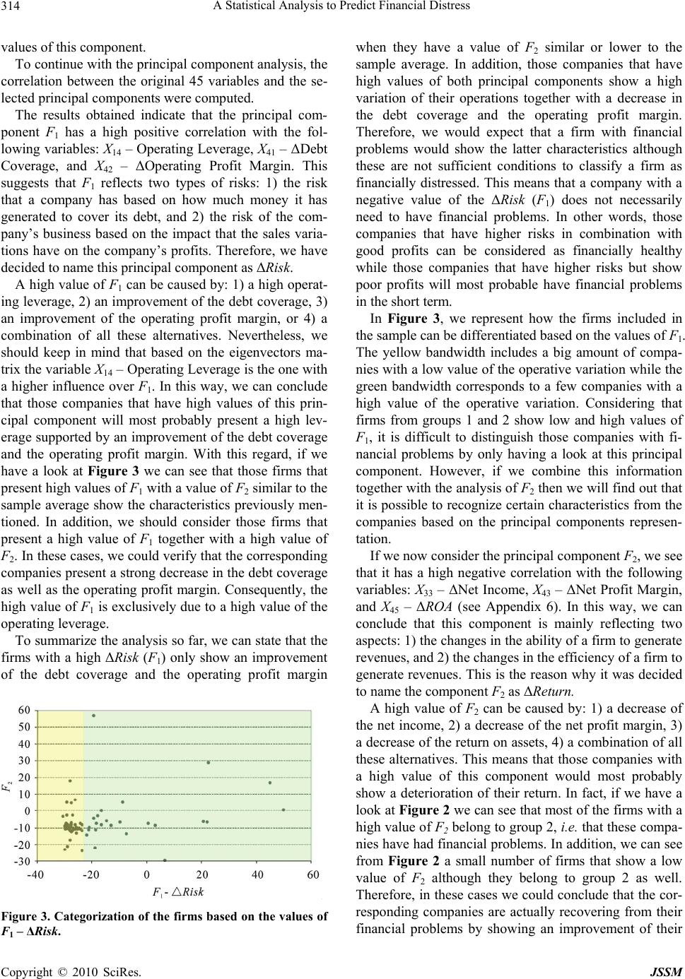

A Statistical Analysis to Predict Financial Distress 314
values of this component.
To continue with the principal component analysis, the
correlation between the original 45 variables and the se-
lected principal components were computed.
The results obtained indicate that the principal com-
ponent F1 has a high positive correlation with the fol-
lowing variables: X14 – Operating Leverage, X41 – ΔDebt
Coverage, and X42 – ΔOperating Profit Margin. This
suggests that F1 reflects two types of risks: 1) the risk
that a company has based on how much money it has
generated to cover its debt, and 2) the risk of the com-
pany’s business based on the impact that the sales varia-
tions have on the company’s profits. Therefore, we have
decided to name this principal component as ΔRisk.
A high value of F1 can be caused by: 1) a high operat-
ing leverage, 2) an improvement of the debt coverage, 3)
an improvement of the operating profit margin, or 4) a
combination of all these alternatives. Nevertheless, we
should keep in mind that based on the eigenvectors ma-
trix the variable X14 – Operating Leverage is the one with
a higher influence over F1. In this way, we can conclude
that those companies that have high values of this prin-
cipal component will most probably present a high lev-
erage supported by an improvement of the debt coverage
and the operating profit margin. With this regard, if we
have a look at Figure 3 we can see that those firms that
present high values of F1 with a value of F2 similar to the
sample average show the characteristics previously men-
tioned. In addition, we should consider those firms that
present a high value of F1 together with a high value of
F2. In these cases, we could verify that the corresponding
companies present a strong decrease in the debt coverage
as well as the operating profit margin. Consequently, the
high value of F1 is exclusively due to a high value of the
operating leverage.
To summarize the analysis so far, we can state that the
firms with a high ΔRisk (F1) only show an improvement
of the debt coverage and the operating profit margin
Figure 3. Categorization of the firms based on the values of
F1 – ΔRisk.
when they have a value of F2 similar or lower to the
sample average. In addition, those companies that have
high values of both principal components show a high
variation of their operations together with a decrease in
the debt coverage and the operating profit margin.
Therefore, we would expect that a firm with financial
problems would show the latter characteristics although
these are not sufficient conditions to classify a firm as
financially distressed. This means that a company with a
negative value of the ΔRisk (F1) does not necessarily
need to have financial problems. In other words, those
companies that have higher risks in combination with
good profits can be considered as financially healthy
while those companies that have higher risks but show
poor profits will most probable have financial problems
in the short term.
In Figure 3, we represent how the firms included in
the sample can be differentiated based on the values of F1.
The yellow bandwidth includes a big amount of compa-
nies with a low value of the operative variation while the
green bandwidth corresponds to a few companies with a
high value of the operative variation. Considering that
firms from groups 1 and 2 show low and high values of
F1, it is difficult to distinguish those companies with fi-
nancial problems by only having a look at this principal
component. However, if we combine this information
together with the analysis of F2 then we will find out that
it is possible to recognize certain characteristics from the
companies based on the principal components represen-
tation.
If we now consider the principal component F2, we see
that it has a high negative correlation with the following
variables: X33 – ΔNet Income, X43 – ΔNet Profit Margin,
and X45 – ΔROA (see Appendix 6). In this way, we can
conclude that this component is mainly reflecting two
aspects: 1) the changes in the ability of a firm to generate
revenues, and 2) the changes in the efficiency of a firm to
generate revenues. This is the reason why it was decided
to name the component F2 as ΔReturn.
A high value of F2 can be caused by: 1) a decrease of
the net income, 2) a decrease of the net profit margin, 3)
a decrease of the return on assets, 4) a combination of all
these alternatives. This means that those companies with
a high value of this component would most probably
show a deterioration of their return. In fact, if we have a
look at Figure 2 we can see that most of the firms with a
high value of F2 belong to group 2, i.e. that these compa-
nies have had financial problems. In addition, we can see
from Figure 2 a small number of firms that show a low
value of F2 although they belong to group 2 as well.
Therefore, in these cases we could conclude that the cor-
responding companies are actually recovering from their
financial problems by showing an improvement of their

A Statistical Analysis to Predict Financial Distress 315
returns.
In Figure 4, we represent how the firms included in
the sample can be differentiated based on the values of F2.
The red bandwidth includes those companies that have
shown a high deterioration of their returns while the
green bandwidth corresponds to those firms that have
shown an improvement in their returns. In addition, we
have defined a yellow bandwidth that corresponds to
those companies that show a similar value of their ΔReturn
that approximates to the sample average.
After performing an analysis of each principal com-
ponent, we can now combine all the information obtained
to define different clusters that can help us to identify the
status of a certain firm with regard to its ΔRisk and
ΔReturn. This classification of the sample is represented
in Figure 5 together with a description of the type of
evolution that a company belonging to a certain sector
has suffered.
Figure 4. Categorization of the firms based on the values of
F2 – ΔReturn.
Figure 5. Categorization of the firms based on the principal
components.
We would expect those firms with a higher disposition
to have financial problems in the short term to fall into
sectors 1 or 2. The sector 1 corresponds to firms showing
a significant deterioration on their returns while sector 2
represents companies showing higher risks in combina-
tion with a deterioration of their returns. In a similar way,
we would expect those firms with a low disposition to
have financial problems in the short term to fall into sec-
tors 5 or 6. The sector 5 corresponds to those companies
that show signs of stability, low risk and return im-
provement. In a similar way, the sector 6 is represented
by companies that show a significant return increase in
combination with higher risks. In the case of sectors 3
and 4 it is not possible to link them to any of the groups
considered, i.e. that for those companies falling into these
sectors we are not able to make any conclusions with
regard to their disposition of having financial problems
in the near future. We could say that these companies
have a financial situation similar to the sample average.
However, we should keep in mind that those companies
within sector 4 have higher risks in comparison to those
firms from sector 3.
To summarize, we have seen that the results obtained
after performing the principal component analysis indi-
cate that this technique has been very useful to achieve a
better representation of the firms, especially considering
the power of synthesis that it brings by compiling the
information contained in the 45 original variables into
only 2 new components. By the computation of these
new variables it is possible to quickly financially catego-
rize a certain firm based on the risk the company has
with regard to the nature of its business and the risk in-
volved in the amount of debt it has taken in comparison
to the profits that were generated during the last two fis-
cal years. In this way, depending on the sector to which a
company belongs to it is possible—in some cases—to
make an inference with regard to the disposition of this
firm to have financial problems in the short term. In the
next section, we will perform a logistics regression ana-
lysis to develop a statistical model that allows us to esti-
mate the probability that a firm becomes financially dis-
tressed in the short term. In this way, we will be able to
compute a new quantitative measure that will help us to
identify those firms with financial problems.
5. Logistics Regression Analysis
Because the principal components F1 – ΔRisk and F2 –
ΔReturn have been useful to represent the firms from the
sample and because they hold 93% of the total variance
from the 45 original variables included in the analysis, it
would be reasonable to use these components to build a
logistics regression model. To do this we followed the
procedures proposed by Hosmer and Lemeshow [10]. In

A Statistical Analysis to Predict Financial Distress 316
this way, this model would allow us to estimate the proba-
bility that a firm becomes financially distressed in the
short term, which in the end could be used as a quantita-
tive measure to help us to identify those companies with
financial problems. However, the results obtained from
the model validation based on the coefficients of deter-
mination indicate that the model only explains a small
percentage (31.87%) of the behavior of the dependant
variable we are trying to estimate: Y – Financial Distress
(Y = 1 if the firm IS financially distressed, Y = 0 if the
firm is NOT financially distressed). Therefore, we de-
cided to further investigate if it is possible to find a re-
gression model that can better adjust to the data collected.
If we keep in mind that the principal components are
actually a linear combination of the 45 ratios considered
in this study, we could then make the following question:
What would happen if we develop a regression model
only with those ratios that are representative of each prin-
cipal component? The reason of this question is that the
variance of each principal component can be negatively
affected by the values of some ratios that are not useful
to identify those firms with financial problems. This does
not mean that the regression model based on the principal
components is useless but it brings the opportunity of
finding a new model that better explains the behavior of
the firms in the sample.
To answer our question, we decided to build a new re-
gression model based only on those ratios that have a me-
dium or high correlation with the principal component F2
– ΔReturn. In this case, the result obtained from the
model validation indicates that this group of ratios can
explain 35.63% of the variance of the dependant variable
Y – Financial Distress. In this way, we verified the idea
that the new model is more efficient to identify those
firms with financial problems in comparison to the prin-
cipal components model. This is because we can obtain
similar results but with much more less information.
Therefore, following this reasoning, we can state that al-
though the principal components analysis has been useful
to represent companies with different financial profiles it
is not effective to use these results in a regression model.
In fact, we have demonstrated that with a few ratios we
can develop a model that manages to identify a similar
percentage as the model based on the principal compo-
nents, which contains data collected from all the 45 ratios.
To summarize, we have demonstrated that in this par-
ticular study it is difficult to combine the principal com-
ponent and the logistic regression analyses. This situation
brings us a new problem. It might be the case that there
are some ratios that are effective to estimate the prob-
ability that a firm becomes financially distressed in the
short term but that they have a low correlation with the
principal components. To solve this problem, it was de-
cided to carry out a global analysis that contemplates the
45 financial ratios included in this study.
It is clear that if we consider all the possible combina-
tions that can be obtained based on the 45 ratios to de-
velop a regression model with no more than 5 variables
then it would be very hard to evaluate and compare all
these alternatives by trial and error. Because of this rea-
son, we decided to implement a methodology that allows
us to reduce the number of models to be compared. This
methodology consists in focusing our attention on the
first 22 ratios with the highest coefficient of determina-
tion based on a regression model with a single inde-
pendent variable. In this way, the objective is to develop
different models only with those variables that by them-
selves are more effective to identify those firms with
financial problems. It is important to keep in mind that
this methodology does not guarantee an optimal solution.
This is due to the fact that a certain ratio can show a low
R2 in a regression model with a single independent vari-
able but when it is combined with other ratios then the
information that brings to identify those firms with fi-
nancial problems can be much higher. Nevertheless, the
methodology implemented is still a valid procedure to
find a near optimal solution especially if we consider the
high amount of ratios included in the analysis and that
many of these variables are correlated.
In Table 1, we present the ranking of the coefficients
of determination. From these results, we can see that
those variables that had a higher correlation with the prin-
cipal components are spread all over the ranking. How-
ever, we should notice that most of the ratios that are cor-
related with the component F2 have a R2 higher than 0.1.
This could be explained by the fact that the parameter
value from the component F2 in the regression model is
higher than the component F1. In addition, it is important
to mention that most of the ratios that can better individu-
ally explain the behavior of the firms are related to prof-
itability and return aspects.
Based on the first 22 ratios shown in Table 1, a total
of 57 regression models were tested (see Appendix 7).
We should notice that we have not included the outliers
identified in the principal component analysis when de-
veloping any of these logistics regression models. We
limited each model to 5 independent variables at most. In
addition, the ratios were first grouped based on their cor-
relations to avoid including in the same model more than
one ratio that brings the same type of information. For
example, it is not reasonable to include in the same re-
gression model only ratios related to liquidity aspects
given that we would miss some important financial in-
formation from the companies related to aspects such as
operational performance, debt, profit, and growth.
The models tested were compared based on the value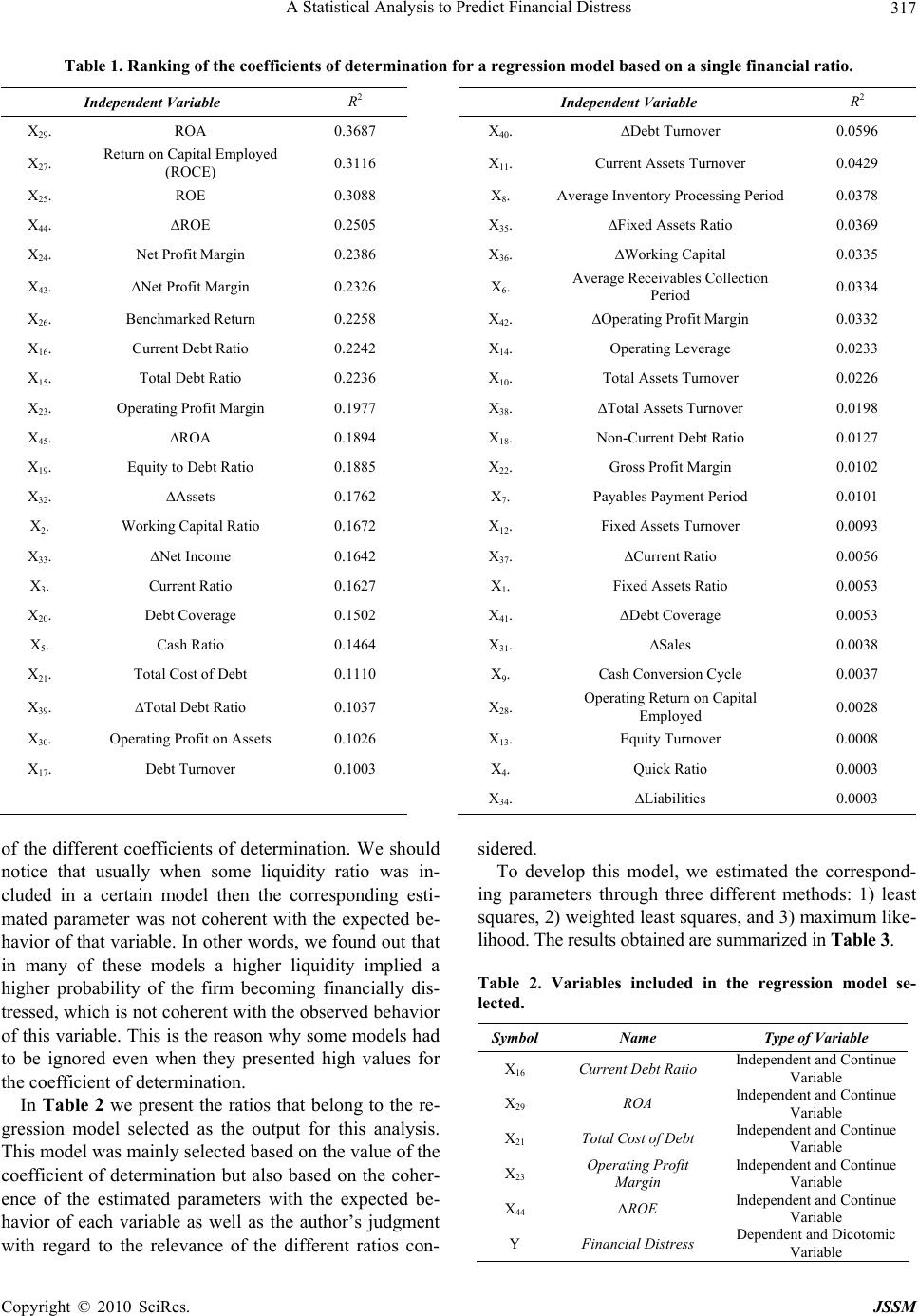

A Statistical Analysis to Predict Financial Distress 317
Table 1. Ranking of the coefficients of determination for a regression model based on a single financial ratio.
Independent Variable R2 Independent Variable R2
X29. ROA 0.3687 X40. ∆Debt Turnover 0.0596
X27. Return on Capital Employed
(ROCE) 0.3116 X11. Current Assets Turnover 0.0429
X25. ROE 0.3088 X8. Average Inventory Processing Period 0.0378
X44. ∆ROE 0.2505 X35. ∆Fixed Assets Ratio 0.0369
X24. Net Profit Margin 0.2386 X36. ∆Working Capital 0.0335
X43. ∆Net Profit Margin 0.2326 X6. Average Receivables Collection
Period 0.0334
X26. Benchmarked Return 0.2258 X42. ∆Operating Profit Margin 0.0332
X16. Current Debt Ratio 0.2242 X14. Operating Leverage 0.0233
X15. Total Debt Ratio 0.2236 X10. Total Assets Turnover 0.0226
X23. Operating Profit Margin 0.1977 X38. ∆Total Assets Turnover 0.0198
X45. ∆ROA 0.1894 X18. Non-Current Debt Ratio 0.0127
X19. Equity to Debt Ratio 0.1885 X22. Gross Profit Margin 0.0102
X32. ∆Assets 0.1762 X7. Payables Payment Period 0.0101
X2. Working Capital Ratio 0.1672 X12. Fixed Assets Turnover 0.0093
X33. ∆Net Income 0.1642 X37. ∆Current Ratio 0.0056
X3. Current Ratio 0.1627 X1. Fixed Assets Ratio 0.0053
X20. Debt Coverage 0.1502 X41. ∆Debt Coverage 0.0053
X5. Cash Ratio 0.1464 X31. ∆Sales 0.0038
X21. Total Cost of Debt 0.1110 X9. Cash Conversion Cycle 0.0037
X39. ∆Total Debt Ratio 0.1037 X28. Operating Return on Capital
Employed 0.0028
X30. Operating Profit on Assets 0.1026 X13. Equity Turnover 0.0008
X17. Debt Turnover 0.1003 X4. Quick Ratio 0.0003
X34. ∆Liabilities 0.0003
of the different coefficients of determination. We should
notice that usually when some liquidity ratio was in-
cluded in a certain model then the corresponding esti-
mated parameter was not coherent with the expected be-
havior of that variable. In other words, we found out that
in many of these models a higher liquidity implied a
higher probability of the firm becoming financially dis-
tressed, which is not coherent with the observed behavior
of this variable. This is the reason why some models had
to be ignored even when they presented high values for
the coefficient of determination.
In Table 2 we present the ratios that belong to the re-
gression model selected as the output for this analysis.
This model was mainly selected based on the value of the
coefficient of determination but also based on the coher-
ence of the estimated parameters with the expected be-
havior of each variable as well as the author’s judgment
with regard to the relevance of the different ratios con-
sidered.
To develop this model, we estimated the correspond-
ing parameters through three different methods: 1) least
squares, 2) weighted least squares, and 3) maximum like-
lihood. The results obtained are summarized in Table 3.
Table 2. Variables included in the regression model se-
lected.
Symbol Name Type of Variable
X16 Current Debt Ratio Independent and Continue
Variable
X29 ROA Independent and Continue
Variable
X21 Total Cost of Debt Independent and Continue
Variable
X23 Operating Profit
Margin
Independent and Continue
Variable
X44 ∆ROE Independent and Continue
Variable
Y Financial Distress Dependent and Dicotomic
Variable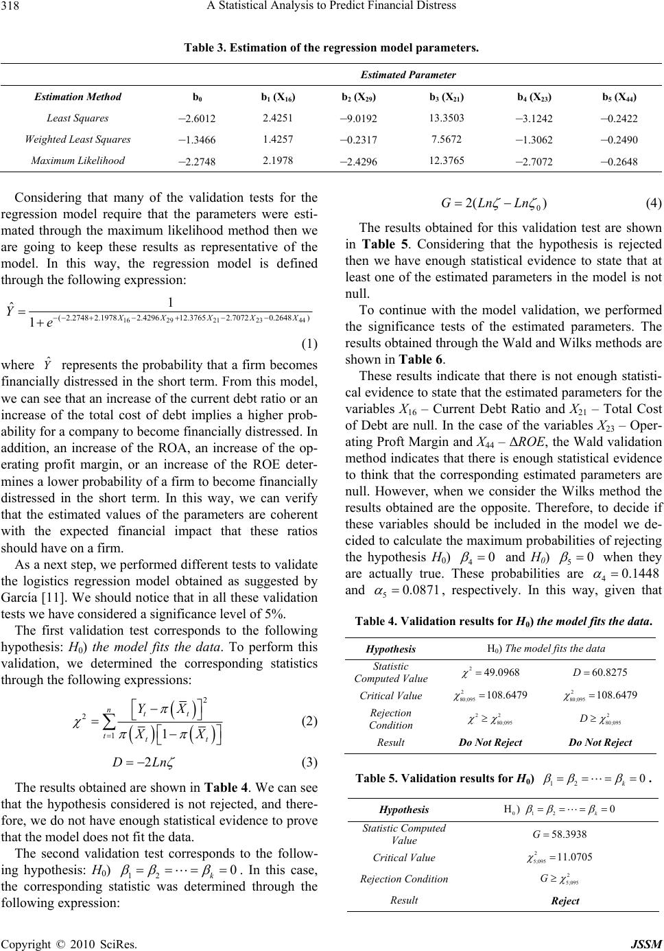

A Statistical Analysis to Predict Financial Distress 318
Table 3. Estimation of the regression model parameters.
Estimated Parameter
Estimation Method b0 b1 (X16) b2 (X29) b3 (X21) b4 (X23) b5 (X44)
Least Squares –2.6012 2.4251 –9.0192 13.3503 –3.1242 –0.2422
Weighted Least Squares –1.3466 1.4257 –0.2317 7.5672 –1.3062 –0.2490
Maximum Likelihood –2.2748 2.1978 –2.4296 12.3765 –2.7072 –0.2648
Considering that many of the validation tests for the
regression model require that the parameters were esti-
mated through the maximum likelihood method then we
are going to keep these results as representative of the
model. In this way, the regression model is defined
through the following expression:
162921 23 44
( 2.2748 2.19782.429612.37652.70720.2648)
1
ˆ
1XX XXX
Ye  
(1)
where represents the probability that a firm becomes
financially distressed in the short term. From this model,
we can see that an increase of the current debt ratio or an
increase of the total cost of debt implies a higher prob-
ability for a company to become financially distressed. In
addition, an increase of the ROA, an increase of the op-
erating profit margin, or an increase of the ROE deter-
mines a lower probability of a firm to become financially
distressed in the short term. In this way, we can verify
that the estimated values of the parameters are coherent
with the expected financial impact that these ratios
should have on a firm.
Y
ˆ
As a next step, we performed different tests to validate
the logistics regression model obtained as suggested by
García [11]. We should notice that in all these validation
tests we have considered a significance level of 5%.
The first validation test corresponds to the following
hypothesis: H0) the model fits the data. To perform this
validation, we determined the corresponding statistics
through the following expressions:

 
2
2
11
ntt
ttt
YX
XX









 (2)
2DLn

 (3)
The results obtained are shown in Table 4. We can see
that the hypothesis considered is not rejected, and there-
fore, we do not have enough statistical evidence to prove
that the model does not fit the data.
The second validation test corresponds to the follow-
ing hypothesis: H0) 12 0
k

 . In this case,
the corresponding statistic was determined through the
following expression:
0
2( )GLnLn


 (4)
The results obtained for this validation test are shown
in Table 5. Considering that the hypothesis is rejected
then we have enough statistical evidence to state that at
least one of the estimated parameters in the model is not
null.
To continue with the model validation, we performed
the significance tests of the estimated parameters. The
results obtained through the Wald and Wilks methods are
shown in Table 6.
These results indicate that there is not enough statisti-
cal evidence to state that the estimated parameters for the
variables X16 – Current Debt Ratio and X21 – Total Cost
of Debt are null. In the case of the variables X23 – Oper-
ating Proft Margin and X44 – ΔROE, the Wald validation
method indicates that there is enough statistical evidence
to think that the corresponding estimated parameters are
null. However, when we consider the Wilks method the
results obtained are the opposite. Therefore, to decide if
these variables should be included in the model we de-
cided to calculate the maximum probabilities of rejecting
the hypothesis H0) 40


and H0) 50

 when they
are actually true. These probabilities are 40.1448


and 50.0871


, respectively. In this way, given that
Table 4. Validation results for H0) the model fits the data.
Hypothesis H0) The model fits the data
Statistic
Computed Value
249.0968
  60.8275D
Critical Value 2
80;095 108.6479
  2
80;095 108.6479
 
Rejection
Condition
22
80;095
  2
80;095
D  
Result Do Not Reject Do Not Reject
Table 5. Validation results for H0) 12 0
k

 .
Hypothesis 01 2
H) 0
k
  
Statistic Computed
Value 58.3938G
Critical Value 2
5;095 11.0705
 
Rejection Condition 2
5;095
G  
Result Reject

A Statistical Analysis to Predict Financial Distress 319
Table 6. Validation results for the significance tests of the estimated parameters.
Estimated Parameters
Wald Method b1 (X16) b2 (X29) b3 (X21) b4 (X23) b5 (X44)
Hypothesis 01
H) 0   02 H) 0 

03 H) 0 

04 H) 0   05 H) 0 

Statistic Computed
Value 2.2064t 0.5036t 1.6817t

1.0661t

 1.3713t
Critical Value 80;0.95 1.6641t 80;0.95 1.6641t 80;0.95 1.6641t 80;0.95 1.6641t 80;0.95 1.6641t
Rejection Condition 80;0.95
tt 80;0.95 tt 80;0.95 tt 80;0.95 tt 80;0.95 tt
Result Reject Do Not Reject Reject Do Not Reject Do Not Reject
Estimated Parameters
Wilks Method b1 (X16) b2 (X29) b3 (X21) b4 (X23) b5 (X44)
Hypothesis 01
H) 0   02 H) 0 

03 H) 0 

04 H) 0   05 H) 0 

Statistic Computed
Value
29.7588
  20.3969   24.4051   24.2093   26.6551  
Critical Value 2
1;0.9 2.7055
  2
1;0.9 2.7055
  2
1;0.9 2.7055
  2
1;0.9 2.7055
  2
1;0.9 2.7055
 
Rejection Condition 22
1;0.9

  22
1;0.9

  22
1;0.9

  22
1;0.9

  22
1;0.9

 
Result Reject Do Not Reject Reject Reject Reject
these probabilities are quite low, we concluded that there
is not enough statistical evidence to think that the esti-
mated parameters of the variables X23 and X44 are null.
Finally, we need to consider the estimated parameter
associated with the variable X29 – ROA. In this case, the
hypothesis H0) 20


2
is not being rejected in the Wald
validation method nor in the Wilks method. In fact, the
maximum probability of rejecting this hypothesis when it
is actually true is 0.308


0.528
according to the Wald’s
statistic and 27

 according to the Wilks’ statis-
tic. These results indicate that there is enough statistical
evidence to believe that the corresponding variable
should not be included in the regression model given that
it does not help to identify those firms with financial
problems. To verify this statement we compared the re-
gression model that includes the variable X29 – ROA
against that model that does not include this ratio based
on the coefficients of determination and the ability of
each model to identify a firm with financial problems1.
The results obtained—as shown in Tables 7 and 8—
indicate that the additional information provided by the
variable X29 – ROA is negligible, and therefore, we have
decided not to include this variable in the regression mo-
del.
To finalize with the validation process, we can analyze
the results obtained in Tables 7 and 8. The most impor-
tant thing to notice is the improvement that the model
based on the original variables shows in comparison to
the model based on the principal components. If we have
a look at the coefficients of determination then the
maximum value obtained for the model based on the
original variables is 0.654 while for the model based on
the principal components is 0.3187. In a similar way, the
model based on the original variables managed to cor-
rectly identify 84.88% of the firms—either as a firm with
or without financial problems—while the principal com-
ponents model correctly identified 78.57% of the firms in
the sample. All in all, these validation metrics reflect the
robustness of the regression model selected.
Given that from the model validation we concluded
that the variable X29 – ROA should not be considered, the
new regression model can be represented as follows:
1621 23 44
( 2.4567 2.281314.23153.5630.271)
1
ˆ
1XXXX
Ye   (5)
where the parameters corresponding to each financial
ratio were again estimated through the maximum likeli-
hood method. As in the previous model, the relation be-
tween the estimated parameters and the variables consid-
ered is coherent as we can see from Expression (5).
The validation of this new model is quite straight for-
ward since we only left out one financial ratio in com-
parison to the previous model. As in previous validations,
first we tested the hypothesis H0) the model fits the data
and we found that there was not enough statistical evi-
dence to reject it. Second, we tested the hypothesis H0)
12 0 k



  and in this case we found out that
there was enough statistical evidence to state that not all
the estimated parameters are null. To continue with the
validation process we also performed the significance
tests of the regression coefficients. The results obtained
are shown in Table 9. In this case, we can see that

A Statistical Analysis to Predict Financial Distress 320
Table 7. Comparison of the coefficients of determination.
Regression Model based on X16, X29, X21, X23, and X4 Regression Model based on X16, X21, X23, and X44
Coefficients of Determination Value Coefficients of Determination Value
2
R
0.5858 2
R
0.5504
2
M
cFadden
R 0.4898 2
M
cFadden
R 0.4865
2
A
ldrich Nelson
R 0.4044 2
A
ldrich Nelson
R 0.4028
2
Cox Snell
R 0.4929 2
Cox Snell
R 0.4905
2
ker
Nagel ke
R 0.6572 2
ker
Nagel ke
R 0.6540
Table 8. Comparison of the ability of the models to identify a firm with financial problems.
Regression Model based on X16, X29, X21, X23, and X44 Regression Model based on X16, X21, X23, and X44
Correct
Classifications
Incorrect
Classifications Total Correct Classifications
Incorrect
Classifications Total
Group 1 97.67% 2.33% 100% Group 1 95.35% 4.65% 100%
Group 2 76.74% 23.26% 100% Group 2 74.42% 25.58% 100%
Total 87.21% 12.79% 100% Total 84.88% 15.12% 100%
Table 9. Validation results for the significance tests of the estimated parameters.
Estimated Parameters
Wald Method b1 (X16) b3 (X21) b4 (X23) b5 (X44)
Hypothesis 01
H) 0   03 H) 0 

04 H) 0 

05 H) 0  
Statistic Computed Value 2.3395t 2.1002t 1.6862t 1.7514t
Critical Value 81;0.95 1.6639t 81;0.95 1.6639t 81;0.95 1.6639t 81;0.95 1.6639t
Rejection Condition 81;0.95
tt 81;0.95 tt 81;0.95 tt 81;0.95 tt
Result Reject Reject Reject Reject
Estimated Parameters
Wilks Method b1 (X16) b3 (X21) b4 (X23) b5 (X44)
Hypothesis 01
H) 0   03 H) 0 

04 H) 0 

05 H) 0  
Statistic Computed Value 29.8813
  26.4451   26.4641   215.2369  
Critical Value 2
1;0.9 2.7055
  2
1;0.9 2.7055
  2
1;0.9 2.7055
  2
1;0.9 2.7055
 
Rejection Condition 22
1;0.9

  22
1;0.9

  22
1;0.9

  22
1;0.9

 
Result Reject Reject Reject Reject
every hypothesis tested H0) 0
i

 is rejected through
both the Wald and Wilks methods, being the validation
results more robust that in the previous regression model
validation.
The validation concludes with the calculation of the
coefficients of determination and the ability of the model
to correctly classify the firms in the sample, which were
already presented in Tables 7 and 8, respectively. In this
way, we can finish with the regression analysis by com-
puting the 95% confidence intervals for each of the esti-
mated parameters from the selected regression model.
The results obtained are the following:
12.2813 1.9407


 (6)
314.2315 13.4856


 (7)
43.563 4.2052


 (8)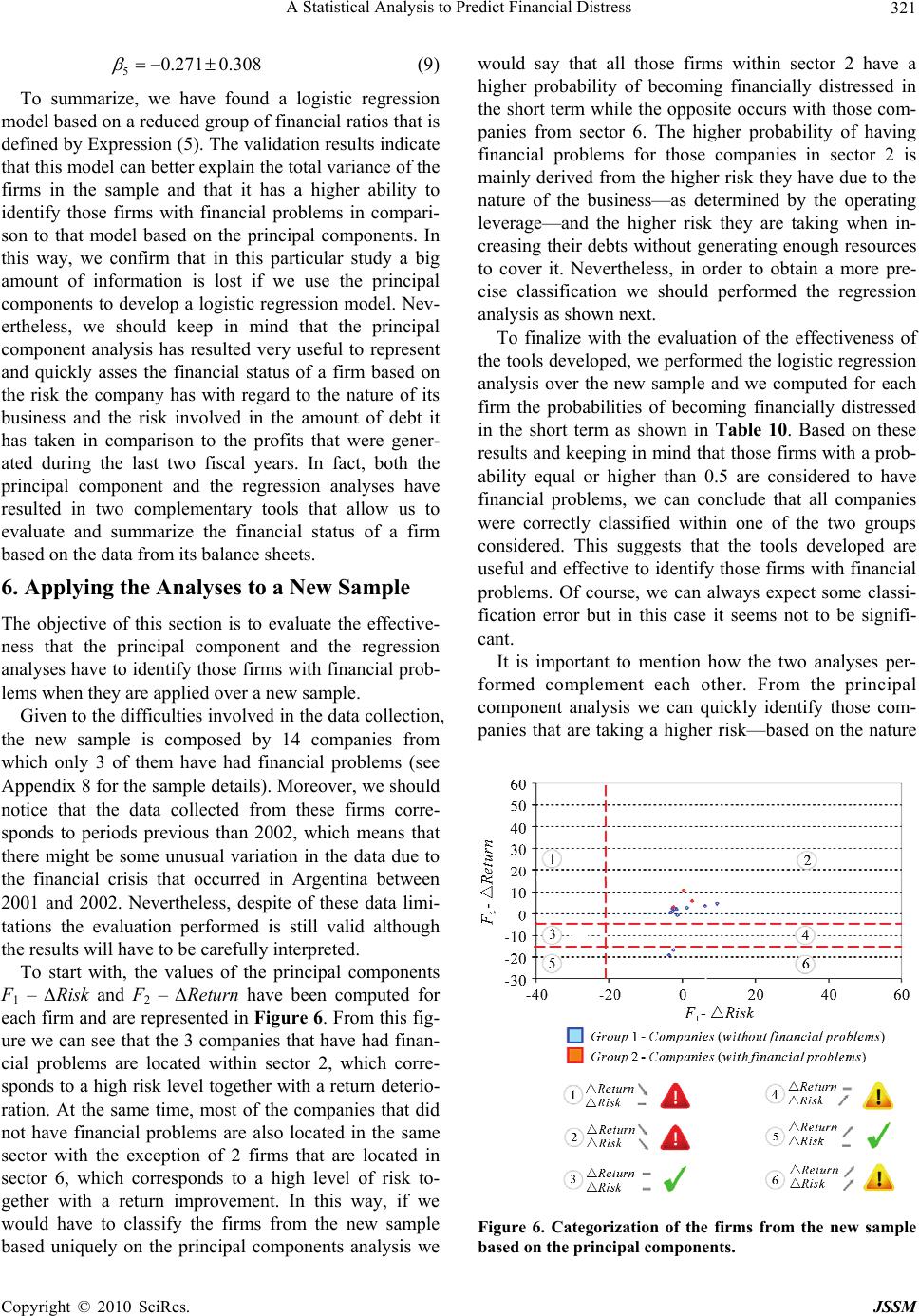

A Statistical Analysis to Predict Financial Distress 321
50.271 0.308

  (9)
To summarize, we have found a logistic regression
model based on a reduced group of financial ratios that is
defined by Expression (5). The validation results indicate
that this model can better explain the total variance of the
firms in the sample and that it has a higher ability to
identify those firms with financial problems in compari-
son to that model based on the principal components. In
this way, we confirm that in this particular study a big
amount of information is lost if we use the principal
components to develop a logistic regression model. Nev-
ertheless, we should keep in mind that the principal
component analysis has resulted very useful to represent
and quickly asses the financial status of a firm based on
the risk the company has with regard to the nature of its
business and the risk involved in the amount of debt it
has taken in comparison to the profits that were gener-
ated during the last two fiscal years. In fact, both the
principal component and the regression analyses have
resulted in two complementary tools that allow us to
evaluate and summarize the financial status of a firm
based on the data from its balance sheets.
6. Applying the Analyses to a New Sample
The objective of this section is to evaluate the effective-
ness that the principal component and the regression
analyses have to identify those firms with financial prob-
lems when they are applied over a new sample.
Given to the difficulties involved in the data collection,
the new sample is composed by 14 companies from
which only 3 of them have had financial problems (see
Appendix 8 for the sample details). Moreover, we should
notice that the data collected from these firms corre-
sponds to periods previous than 2002, which means that
there might be some unusual variation in the data due to
the financial crisis that occurred in Argentina between
2001 and 2002. Nevertheless, despite of these data limi-
tations the evaluation performed is still valid although
the results will have to be carefully interpreted.
To start with, the values of the principal components
F1 – ∆Risk and F2 – ∆Return have been computed for
each firm and are represented in Figure 6. From this fig-
ure we can see that the 3 companies that have had finan-
cial problems are located within sector 2, which corre-
sponds to a high risk level together with a return deterio-
ration. At the same time, most of the companies that did
not have financial problems are also located in the same
sector with the exception of 2 firms that are located in
sector 6, which corresponds to a high level of risk to-
gether with a return improvement. In this way, if we
would have to classify the firms from the new sample
based uniquely on the principal components analysis we
would say that all those firms within sector 2 have a
higher probability of becoming financially distressed in
the short term while the opposite occurs with those com-
panies from sector 6. The higher probability of having
financial problems for those companies in sector 2 is
mainly derived from the higher risk they have due to the
nature of the business—as determined by the operating
leverage—and the higher risk they are taking when in-
creasing their debts without generating enough resources
to cover it. Nevertheless, in order to obtain a more pre-
cise classification we should performed the regression
analysis as shown next.
To finalize with the evaluation of the effectiveness of
the tools developed, we performed the logistic regression
analysis over the new sample and we computed for each
firm the probabilities of becoming financially distressed
in the short term as shown in Table 10. Based on these
results and keeping in mind that those firms with a prob-
ability equal or higher than 0.5 are considered to have
financial problems, we can conclude that all companies
were correctly classified within one of the two groups
considered. This suggests that the tools developed are
useful and effective to identify those firms with financial
problems. Of course, we can always expect some classi-
fication error but in this case it seems not to be signifi-
cant.
It is important to mention how the two analyses per-
formed complement each other. From the principal
component analysis we can quickly identify those com-
panies that are taking a higher risk—based on the nature
Figure 6. Categorization of the firms from the new sample
based on the principal components.

A Statistical Analysis to Predict Financial Distress 322
Table 10. Probabilities for a firm to become financially dis-
tressed in the short term.
Firm Nr Group Nr Probability
1 1 0.0045
2 1 0.2164
3 1 0.1569
4 1 0.3691
5 1 0.2479
6 1 0.0863
7 1 0.2680
8 1 0.4766
9 1 0.1244
10 1 0.3013
11 1 0.2462
12 2 0.5593
13 2 0.7444
14 2 0.5279
of the business and based on the higher debts—and to
identify those companies that have a better coverage
against that risk. From the regression analysis we are
able to quantify through a unique indicator—the prob-
ability of becoming financially distressed in the short
term—how big is the risk involved and how good is the
company covering against that risk. In addition, we can
use this probability to identify those firms that already
have financial problems.
7. Conclusions
Through this study we managed to verify based on the
statistical analyses performed that the financial ratios
show a different behavior between those firms that have
had financial problems and those which did not. Al-
though not all these ratios have by themselves the same
ability to allow the identification of those firms with fi-
nancial problems, it is possible to combine and summa-
rize all that information into 2 principal components that
we have named as ∆Risk and ∆Return. By the computa-
tion of these new variables it is possible to quickly finan-
cially categorize a certain firm based on the risk the
company has with regard to the nature of its business and
the risk involved in the amount of debt it has taken in
comparison to the profits that were generated during the
last two fiscal years.
The conclusive results obtained from the principal
component analysis suggest that there would be no ap-
parent reason not to consider any financial ratio origi-
nally collected to estimate the probability that a firm be-
comes financially distressed in the short term. However,
after developing different regression models we have
seen that we can obtain better estimations of these prob-
abilities if we just consider a few financial ratios that all
together show a higher ability to identify a firm with fi-
nancial problems in comparison to a situation where the
data collected from all the 45 ratios is used (as in the case
of the principal components model). In this way, we
managed to develop a more efficient model given that we
can obtain better results with less data. This efficiency
can be explained due to the fact that the principal com-
ponents are a linear combination of 45 ratios, which
means that many of them might not be useful to distin-
guish between a financially healthy firm and one that it is
not. This finding shows how important is to have a com-
plete and broad database before starting any statistical
analysis so that fewer limitations are introduced when
trying to find a near optimal solution, i. e. the regression
model with the available ratios combination that best
estimates the probability of a firm of becoming finan-
cially distressed in the short term. In the same way, we
should emphasis the benefits that can be obtained when
combining more than one statistical analysis together to
better understand the nature of the process under study
and to more effectively achieve the objective proposed,
which in our case is to identify those firms with financial
problems.
We have seen that those ratios that have more capa-
bilities to identify those firms with financial problems are
all related to the return aspects of the companies. In fact,
we have seen that the principal component that resulted
more conclusive to identify financially unhealthy firms
was the ∆Return as opposite to the ∆Risk component.
Nevertheless, the information contained in these ratios
can always be complemented with information from
other type of ratios to identify those firms with financial
problems more precisely and effectively. After perform-
ing a logistic regression analysis based on the 45 ratios
collected in the sample, we have selected a small group
of them that can explain 65% of the firms’ behavior. The
related model consists of the following ratios: 1) Current
Debt Ratio, 2) Total Cost of Debt, 3) Operating Profit
Margin, and 4) ∆ROE. It is interesting to notice that in
most of the logistic regression models tested it was found
that there is higher probability to incorrectly classify a
firm with financial problems, i.e. to assume that a com-
pany is financially healthy when actually it is not. This
could be mainly explained due to the fact that the finan-
cial ratios collected have a higher variability in those

A Statistical Analysis to Predict Financial Distress 323
companies that are financially distressed in comparison
to those that do not have any financial problem. Never-
theless, the possibility of combining the regression and
the principal component analyses helps to reduce the
probability of misclassifying a certain firm. With this
regard, we should notice that the present study does not
include any analysis related to the costs involved in the
decision making process of identifying firms with finan-
cial problems. Nevertheless, whenever there are not con-
clusive results that clear define the financial status of a
company then the most conservative decision would be
to assume that the firm has financial problems.
The outcomes from this study are two tools that were
developed based on the statistical inference from which
we can quickly asses the financial status of a firm based
on its risks and return’s variation as well as to estimate
the probability that a firm becomes financially distressed
in the short term. There are different ways of taking these
tools into practice such as: 1) to control and follow up the
financial performance of a company, 2) to support the
decision of lending money to a company, 3) to support
the decision of investing money or the decision of merg-
ing with a company, 4) to support market analysis from a
financial perspective, and 5) to support actions or deci-
sions related to the financial assessment of a company
that declares itself to be financially distressed.
This study could be further developed by trying to in-
corporate new explanatory variables that are rather not
financial ratios but instead qualitative measurements that
could contribute to more precise and effective estimation
of the probability of a firm of becoming financially dis-
tressed in the short term. Another alternative would be to
incorporate a tool from which the costs involved in tak-
ing the wrong decision—i.e. to assume that a company
has no financial problems when it actually has or vice
versa—could be minimized. Finally, the statistical analy-
ses performed in this study could be replicated with firms
that have a significant amount of assets with the objec-
tive of determining the main characteristics that derive in
a solid financial structure. As we can see, there are many
different ways to continue with this study and the statis-
tics offers interesting tools for that.
REFERENCES
[1] I. Guzmán, “Factores explicativos del reparto de divi-
dendos a cuenta en las empresas españolas,” Instituto
Valenciano de Investigaciones Económicas, 2004. http://
www.ivie.es/downloads/docs/wpasec/wpasec-2004-09.pdf
[2] M. L. Heine, “Predicting Financial Distress of Companies:
Revisting the Z-Score and ZETA Models,” Stern School
of Business, New York University, 2000. http://www.stern.
nyu.edu/~ealtman/Zscores.pdf
[3] J. De la Torre Martínez, R. Navarro, A. Azofra and J. C.
Peña, “Aplicación de los modelos SEPARATE y regre-
sión logística para determinar la relevancia de la informa-
ción contable en el mercado de capitales: una com-
paración,” Universidad de Granada, 2002.
[4] M. Kahl, “Financial Distress as a Selection Mechanism:
Evidence from the United States,” Paper 16-01, Anderson
School of Management, University of California, Los An-
geles, 2001. http://repositories.cdlib.org/anderson/fin/16-01
[5] W. H. Beaver, “Financial Ratios as Predictors of Failure,”
Empirical Research in Accounting, selected studies (in
supplement to the Journal of Accounting Research, Janu-
ary, 1967), 1966, pp. 71-111.
[6] E. I. Altman, “Financial Ratios, Discriminant Analysis
and the Prediction of Corporate Bankruptcy,” The Journal
of Finance, Vol. 23, No. 4, 1968, pp. 589-609.
[7] S. S. Alexander, “The Effect of Size of Manufacturing
Corporation on the Distribution of the Rate of Return,”
Review of Economics and Statistics, Vol. 31, No. 3, 1949,
pp. 229-235.
[8] D. Peña, “Análisis de Datos Multivariantes,” McGraw-
Hill, 2002.
[9] D. Johnson, “Métodos Multivariados Aplicados Al Análisis
de Datos,” Thomson, 2000.
[10] D. W. Hosmer and S. Lemeshow, “Applied Logistic Re-
gression,” 2nd Edition, John Wiley & Sons Inc., 2000.
[11] R. M. García, “Inferencia Estadística y Diseño de Experi-
mentos,” Eudeba, 2004.
[12] L. García, “Las Empresas Más Rentables,” Revista Mercado,
2004, pp. 76-80.
[13] L. García, “Las Empresas Más Rentables,” Revista Mercado,
2005, pp. 110-114. http://www.ax5.com/antonio/publica-
ciones/delatorre2002aplicacion.pdf
[14] L. García, “Las 100 Empresas Más Rentables,” Revista Mercado,
2006, pp. 134-138.

A Statistical Analysis to Predict Financial Distress 324
Appendices
Appendix 1
Table A1. Details of the firms included in the sample.
Firm Nr Group Nr Name Period Analyzed Firm’s Industry
1 1 Alvarez Hnos. S.A. 2005-2004 Mills and oils
2 1 Compañía Internacional de Alimentos y Bebidas S.A. 2004-2003 Food
3 1 Establecimiento Metalúrgicos Cavanna S.A.C.I.F.I. 2005-2004 Technology and communications
4 1 Andreani Logística S.A. 2004-2003 Transport
5 1 Compañía de Servicios Telefónicos S.A. 2005-2004 Telecommunications
6 1 Compumundo S.A. 2005-2004 Retail
7 1 Caputo S.A. 2005-2004 Construction
8 1 Ediar S.A. 2005-2004 Printing and publishing
9 1 Agrometal S.A.I. 2005-2004 Machinery and equipment
10 1 Electromac S.A. 2005-2004 Machinery and equipment
11 1 Gijon S.A. 2005-2004 Construction
12 1 Green S.A. 2005-2004 Construction
13 1 Esat S.A. 2004-2003 Plastic and chemical
14 1 Grafex S.A. 2004-2003 Printing and publishing
15 1 Lihue Ingeniería S.A. 2005-2004 Machinery and equipment
16 1 Laboratorio LKM S.A. 2004-2003 Laboratories
17 1 Guilford Argentina S.A. 2005-2004 Textiles and footwear
18 1 Rovella Carranza S.A. 2005-2004 Construction
19 1 Yar Construcciones S.A. 2005-2004 Construction
20 1 Mardi S.A. 2004-2003 Fishing
21 1 Mercoplast S.A. 2005-2004 Plastic and chemical
22 1 Bonafide Golosinas S.A. 2005-2004 Food
23 1 Bonesi S.A. 2005-2004 Household goods
24 1 Molinos Juan Semino S.A. 2004-2003 Mills and oils
25 1 City Pharma S.A. 2005-2004 Retail
26 1 Morixe Hnos. S.A. 2005-2004 Mills and oils
27 1 Coniglio S.A. 2005-2004 Textiles and footwear
28 1 Curtiduría A. Gaita S.R.L. 2005-2004 Tanneries and leather goods
29 1 Domec S.A.I.C. y F. 2005-2004 Household goods
30 1 Dulcor S.A. 2005-2004 Food
31 1 Distribuidora Santa Bárbara S.A. 2005-2004 Fishing
32 1 Outdoors S.A. 2004-2003 Textiles and footwear
33 1 Frutucumán S.A. 2003-2002 Export and import
34 1 García Reguera S.A. 2005-2004 Wholesale
35 1 Instituto Rosenbusch S.A. 2005-2004 Healthcare
36 1 Insumos Agroquímicos S.A. 2005-2004 Retail
37 1 Industria Textil Argentina (INTA) S.A. 2005-2004 Textiles and footwear
38 1 SAT Médica S.A. 2005-2004 Healthcare
39 1 Leyden S.A.I.C. y F. 2005-2004 Machinery and equipment
40 1 Lodge S.A. 2004-2003 Agricultural

A Statistical Analysis to Predict Financial Distress 325
41 1 Longvie S.A. 2005-2004 Household goods
42 1 Ovoprot International S.A. 2004-2003 Food
43 1 Magalcuer S.A. 2005-2004 Tanneries and leather goods
44 2 Aero Vip S.A. 2003-2002 Transport
45 2 Alunamar S.A. 2005-2004 Fishing
46 2 American Falcon S.A. 2003-2002 Transport
47 2 AS Sistemas S.A. 2003-2002 Technology and communications
48 2 Bascoy S.A. 2003-2002 Transport
49 2 Cartex S.A. 2004-2003 Textiles and footwear
50 2 Casamen S.A. 2003-2002 Food
51 2 Celeritas S.A. 2004-2003 Healthcare
52 2 Comercial Mendoza S.A. 2003-2002 Household goods
53 2 Crédito José C. Paz S.A. 2003-2002 Construction
54 2 D´Vigi S.A. 2004-2003 Retail
55 2 Droguería Sigma S.A. 2003-2002 Retail
56 2 Ecourban S.A. 2004-2003 Waste
57 2 El Manzanar de Macedo S.A. 2004-2003 Food
58 2 Espejos Versailles S.A. 2003-2002 Glass and construction materials
59 2 FrigoFruit S.A. 2003-2002 Agricultural
60 2 Humberto Nicolás Fontana S.A.C. 2004-2003 Household goods
61 2 Impresiones Arco Iris Córdoba S.A. 2003-2002 Printing and publishing
62 2 Industrias Badar S.A. 2003-2002 Technology and communications
63 2 Diabolo Menthe S.R.L. 2003-2002 Textiles and footwear
64 2 La Tribu S.R.L. 2003-2002 Food
65 2 Loucen International S.A. 2004-2003 Beverages
66 2 Luicar S.R.L. 2003-2002 Turism
67 2 Manfisa Mandataria y Financiera S.A. 2003-2002 Construction
68 2 Norte Asistencia Empresaria S.A. 2003-2002 Post
69 2 Parmalat Argentina S.A. 2003-2002 Dairy
70 2 Pto. S.A. 2004-2003 Waste
71 2 Redes Excon S.A. 2003-2002 Gas
72 2 Sanatorio Ezeiza S.A. 2004-2003 Healthcare
73 2 Sanatorio Modelo Quilmes S.A. 2004-2003 Healthcare
74 2 Security Consulting S.A. 2003-2002 Technology and communications
75 2 Sepia Beauty S.A. 2004-2003 Cleaning and cosmetics
76 2 Sol de Brasa S.A. 2005-2004 Agricultural
77 2 Sycon Argentina S.A. 2003-2002 Gas
78 2 UOL Sinectis S.A. 2004-2003 Technology and communications
79 2 Yearling S.A. 2003-2002 Security services
80 2 Fundición de Aceros S.A. 2003-2002 Metallurgical and steel
81 2 Inmar S.A. 2003-2002 Construction
82 2 Carpintería Metálica San Eduardo S.A. 2003-2002 Glass and construction materials
83 2 Marmolería Sierra Chica S.A. 2003-2002 Mining
84 2 Avaca S.A. 2003-2002 Textiles and footwear
85 2 Bellas S.A. 2003-2002 Textiles and footwear
86 2 Ianson S.A. 2004-2003 Textiles and footwear

A Statistical Analysis to Predict Financial Distress 326
Appendix 2
Table A2. Description of the financial ratios included in the analyses.
Liquidity Ratios
X1. Fixed Assets Ratio Non Current Assets / Total Assets
X2. Working Capital Ratio Working Capital / Total Assets
X3. Current Ratio Current Assets / Current Liabilities
X4. Quick Ratio (Current Assets - Inventory) / Current Liabilities
X5. Cash Ratio Cash & Equivalents / Current Liabilities
X6. Average Receivables Collection Period Receivables / Sales
X7. Payables Payment Period Accounts Payable / Purchases
X8. Average Inventory Processing Period Average Inventory / COGS
X9. Cash Conversion Cycle Avg. Inventory Processing Period + Avg. Receivables Collection Period - Avg. Payables
Payment Period
Operating Efficiency Ratios
X10. Total Asset Turnover Sales / Total Assets
X11. Current Assets Turnover Sales / Current Assets
X12. Fixed Asset Turnover Sales / Non Current Assets
X13. Equity Turnover Equity / Sales
Business Risk Ratios
X14. Operating Leverage | (%ΔOperating Income) / (%ΔSales) |
Financial Risk Ratios
X15. Total Debt Ratio Total Liabilities / Total Assets
X16. Current Debt Ratio Current Liabilities / Total Assets
X17. Debt Turnover Total Liabilities / Sales
X18. Non Current Debt Ratio Non Current Liabilities / (Non Current Liabilities + Equity)
X19. Equity To Debt Ratio Equity / Total Liabilities
X20. Debt Coverage Operating Profit / Total Liabilities
X21. Total Cost of Debt Interests / Total Liabilities
Return Ratios
X22. Gross Profit Margin Gross Profit / Sales
X23. Operating Profit Margin Operating Profit / Sales
X24. Net Profit Margin Net Income / Sales
X25. Return on Equity (ROE) Net Income / Equity
X26. Benchmarked Return (ROE - ROE sector) / ROE sector
X27. Return on Capital Employed (ROCE) Net Income / (Total Liabilities + Equity)
X28. Operating Return on Capital Employed Operating Profit / (Total Liabilities + Equity)
X29. Return on Assets (ROA) Net Income / Total Assets
X30. Operating Profit on Assets Operating Profit / Total Assets
Growth Ratios
X31. ΔSales (Sales j - Sales j-1) / Sales j-1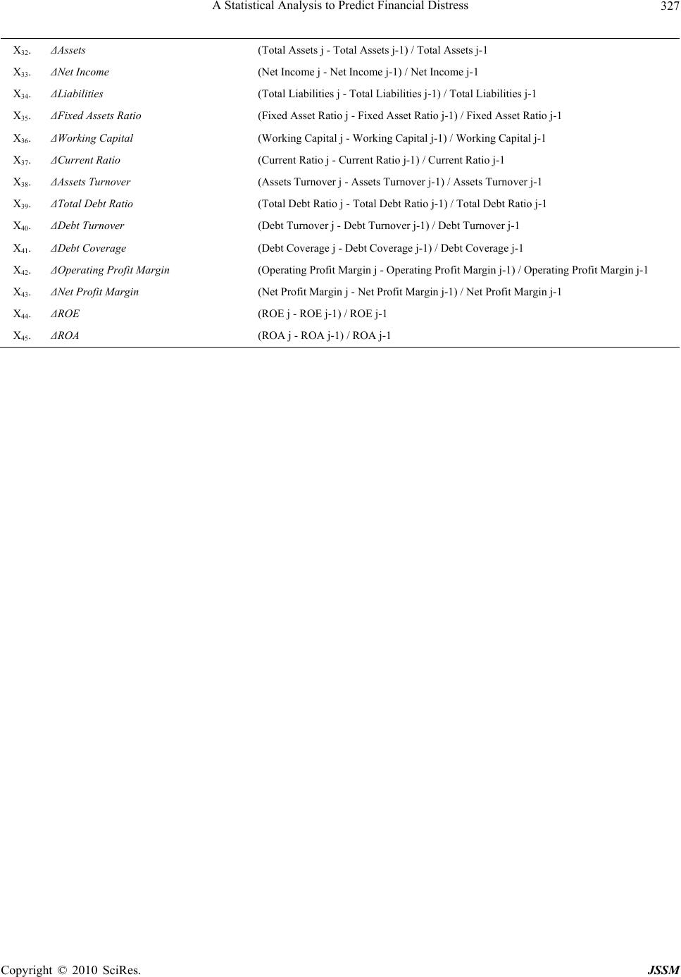

A Statistical Analysis to Predict Financial Distress 327
X32. ΔAssets (Total Assets j - Total Assets j-1) / Total Assets j-1
X33. ΔNet Income (Net Income j - Net Income j-1) / Net Income j-1
X34. ΔLiabilities (Total Liabilities j - Total Liabilities j-1) / Total Liabilities j-1
X35. ΔFixed Assets Ratio (Fixed Asset Ratio j - Fixed Asset Ratio j-1) / Fixed Asset Ratio j-1
X36. ΔWorking Capital (Working Capital j - Working Capital j-1) / Working Capital j-1
X37. ΔCurrent Ratio (Current Ratio j - Current Ratio j-1) / Current Ratio j-1
X38. ΔAssets Turnover (Assets Turnover j - Assets Turnover j-1) / Assets Turnover j-1
X39. ΔTotal Debt Ratio (Total Debt Ratio j - Total Debt Ratio j-1) / Total Debt Ratio j-1
X40. ΔDebt Turnover (Debt Turnover j - Debt Turnover j-1) / Debt Turnover j-1
X41. ΔDebt Coverage (Debt Coverage j - Debt Coverage j-1) / Debt Coverage j-1
X42. ΔOperating Profit Margin (Operating Profit Margin j - Operating Profit Margin j-1) / Operating Profit Margin j-1
X43. ΔNet Profit Margin (Net Profit Margin j - Net Profit Margin j-1) / Net Profit Margin j-1
X44. ΔROE (ROE j - ROE j-1) / ROE j-1
X45. ΔROA (ROA j - ROA j-1) / ROA j-1

A Statistical Analysis to Predict Financial Distress 328
Appendix 3
In Table A3 we present the average ROE per industry based on data published on [12-14]. These average returns have
been used to compute the Benchmarked Return ratio for each company in the sample.
Table A3. Average ROE per industry for companies operating in Argentina.
Year
Firm’s Industry 2003 2004 2005
Agricultural 26.81 29.23 27.02
Household goods 68.18 29.17 39.83
Automotive 31.09 28.27 29.64
Beverages 33.51 34.01 29.01
Pulp and paper 34.75 17.28 18.87 (*)
Wholesale 38.81 36.43 33.44
Retail 51.69 32.95 67.25
Road concessionaire 86.56 (*) 95.16 103.89 (*)
Construction 94.78 47.44 649.63
Post 44.75 48.79 (*) 53.27 (*)
Tanneries and leather goods 42.31 52.54 73.68
Gas 33.24 37.66 28.04
Export and import 43.65 (*) 47.99 52.39 (*)
Finance 257.69 64.35 53.62
Meat 115.63 40.12 43.80 (*)
Oil and gas 128.53 28.81 46.18
Turism 3.24 3.53 (*) 3.86 (*)
Printing and publishing 450.50 33.94 23.91
Fishing 31.19 (*) 34.29 37.43 (*)
Lanoratories 79.01 55.35 60.43
Dairy 39.20 (*) 43.10 87.80
Cleaning and cosmetics 158.33 172.63 (*) 188.48 (*)
Machinery and equipment 124.00 48.32 40.18
Metallurgical and steel 58.72 30.03 31.82
Mining 162.68 22.22 45.05
Mills and oils 74.89 24.18 47.77
Rubber products 28.59 31.17 (*) 28.42
Other 32.61 (*) 35.85 (*) 39.47
Production and distribution of electrical energy 46.30 18.01 56.93
Food 35.35 42.88 38.85
Film Products 14.98 (*) 16.47 17.98 (*)
Plastic and chemical 65.97 18.64 77.78
Chemical and petrochemical 62.35 36.03 36.26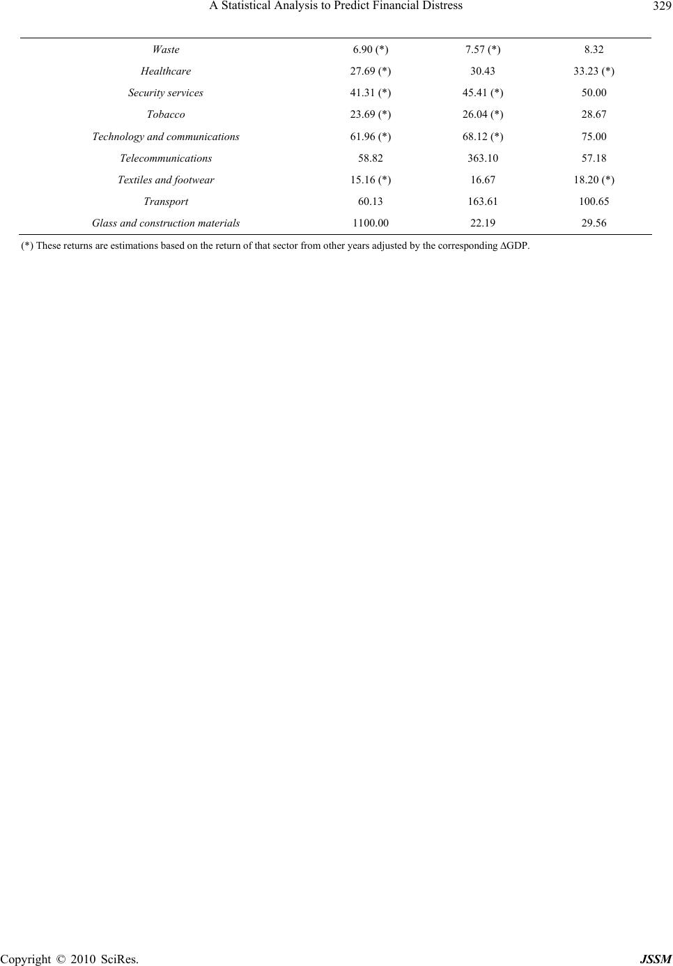

A Statistical Analysis to Predict Financial Distress 329
Waste 6.90 (*) 7.57 (*) 8.32
Healthcare 27.69 (*) 30.43 33.23 (*)
Security services 41.31 (*) 45.41 (*) 50.00
Tobacco 23.69 (*) 26.04 (*) 28.67
Technology and communications 61.96 (*) 68.12 (*) 75.00
Telecommunications 58.82 363.10 57.18
Textiles and footwear 15.16 (*) 16.67 18.20 (*)
Transport 60.13 163.61 100.65
Glass and construction materials 1100.00 22.19 29.56
(*) These returns are estimations based on the return of that sector from other years adjusted by the corresponding ∆GDP.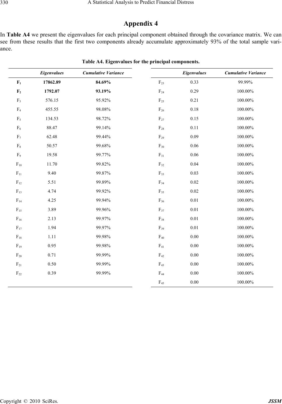

A Statistical Analysis to Predict Financial Distress 330
Appendix 4
In Table A4 we present the eigenvalues for each principal component obtained through the covariance matrix. We can
see from these results that the first two components already accumulate approximately 93% of the total sample vari-
ance.
Table A4. Eigenvalues for the principal components.
Eigenvalues Cumulative Variance Eigenvalues Cumulative Variance
F1 17862.89 84.69%
F23 0.33 99.99%
F2 1792.07 93.19% F24 0.29 100.00%
F3 576.15 95.92% F25 0.21 100.00%
F4 455.55 98.08% F26 0.18 100.00%
F5 134.53 98.72% F27 0.15 100.00%
F6 88.47 99.14% F28 0.11 100.00%
F7 62.48 99.44% F29 0.09 100.00%
F8 50.57 99.68% F30 0.06 100.00%
F9 19.58 99.77% F31 0.06 100.00%
F10 11.70 99.82% F32 0.04 100.00%
F11 9.40 99.87% F33 0.03 100.00%
F12 5.51 99.89% F34 0.02 100.00%
F13 4.74 99.92% F35 0.02 100.00%
F14 4.25 99.94% F36 0.01 100.00%
F15 3.89 99.96% F37 0.01 100.00%
F16 2.13 99.97% F38 0.01 100.00%
F17 1.94 99.97% F39 0.01 100.00%
F18 1.11 99.98% F40 0.00 100.00%
F19 0.95 99.98% F41 0.00 100.00%
F20 0.71 99.99% F42 0.00 100.00%
F21 0.50 99.99% F43 0.00 100.00%
F22 0.39 99.99% F44 0.00 100.00%
F45 0.00 100.00%

A Statistical Analysis to Predict Financial Distress 331
Appendix 5
In Table A5 we present the values that the two principal components selected have in each firm from the sample. Based
on these values, it is possible to represent the firms in a unique graph as shown in Section 4.
Table A5. Values of the principal components for each firm included in the sample.
Firm Nr F1 F2 Firm Nr F1 F2
1 2.89 –8.73
44 –21.32 –11.43
2 –7.46 –13.63 45 –24.91 –10.17
3 –29.61 –9.03 46 –29.61 –8.20
4 –28.65 –9.93 47 –27.52 –12.12
5 –25.48 –11.18 48 –27.59 –8.34
6 –28.02 –9.82 49 –19.58 56.95
7 –24.38 –11.21 50 –27.25 –2.63
8 –29.96 –23.40 51 –10.80 348.78
9 –25.94 –9.77 52 –28.00 77.40
10 6.56 –29.62 53 83.18 –0.38
11 –27.35 –12.27 54 22.53 28.75
12 –13.12 –8.80 55 –24.40 –7.53
13 –26.62 –10.99 56 –19.52 –4.45
14 –27.68 –12.63 57 –16.61 –0.07
15 –21.24 –10.02 58 –27.95 –8.51
16 –9.81 –6.73 59 –29.01 –10.73
17 –29.29 –9.85 60 –29.00 –8.98
18 –28.17 –17.67 61 –18.88 –11.57
19 –29.11 –21.38 62 1,168.66 –28.96
20 21.88 –6.99 63 143.16 65.74
21 –27.91 –9.38 64 –9.03 5.18
22 –23.66 –11.65 65 –23.78 –24.24
23 –29.71 –10.96 66 –29.17 –8.94
24 –28.14 –11.62 67 –18.11 –2.91
25 –29.48 –9.49 68 –28.57 –11.15
26 44.80 16.75 69 –28.76 65.83
27 –26.62 –11.21 70 –25.86 –13.43
28 20.48 –6.61 71 –29.66 –7.74
29 –26.89 –11.24 72 –29.15 –9.30
30 –16.64 –8.22 73 –23.67 –8.33
31 –26.94 –10.14 74 –30.66 –3.28
32 –28.95 –10.66 75 –14.80 –5.93
33 49.83 0.62 76 –26.39 6.42
34 –18.95 –21.99 77 –28.18 17.90
35 –28.73 –10.61 78 –26.25 –8.48
36 –28.63 –9.81 79 –29.34 –2.67
37 –29.95 –9.09 80 –27.60 –7.34
38 –27.47 –11.72 81 –29.40 –7.81
39 –25.99 –10.93 82 296.70 55.26
40 –18.58 –7.64 83 –29.29 –10.68
41 –22.00 –14.59 84 0.38 –7.52
42 –28.22 –11.83 85 –29.25 5.02
43 –29.07 –8.22 86 –27.74 4.48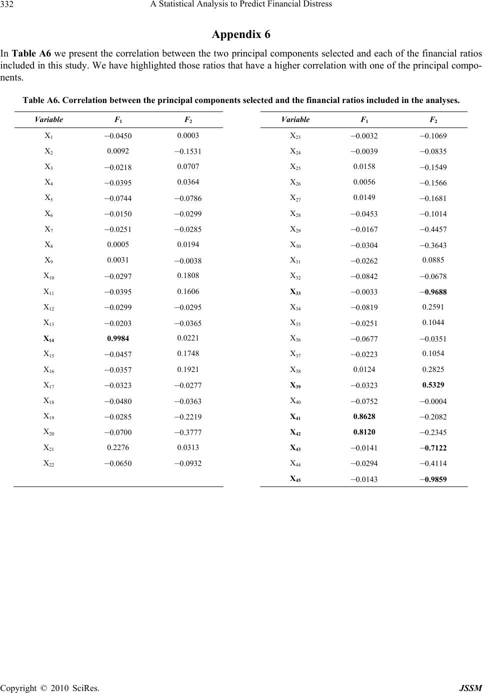

A Statistical Analysis to Predict Financial Distress 332
Appendix 6
In Table A6 we present the correlation between the two principal components selected and each of the financial ratios
included in this study. We have highlighted those ratios that have a higher correlation with one of the principal compo-
nents.
Table A6. Correlation between the principal components selected and the financial ratios included in the analyses.
Variable F1 F2 Variable F1 F2
X1 –0.0450 0.0003 X23 –0.0032 –0.1069
X2 0.0092 –0.1531 X24 –0.0039 –0.0835
X3 –0.0218 0.0707 X25 0.0158 –0.1549
X4 –0.0395 0.0364 X26 0.0056 –0.1566
X5 –0.0744 –0.0786 X27 0.0149 –0.1681
X6 –0.0150 –0.0299 X28 –0.0453 –0.1014
X7 –0.0251 –0.0285 X29 –0.0167 –0.4457
X8 0.0005 0.0194 X30 –0.0304 –0.3643
X9 0.0031 –0.0038 X31 –0.0262 0.0885
X10 –0.0297 0.1808 X32 –0.0842 –0.0678
X11 –0.0395 0.1606 X33 –0.0033 –0.9688
X12 –0.0299 –0.0295 X34 –0.0819 0.2591
X13 –0.0203 –0.0365 X35 –0.0251 0.1044
X14 0.9984 0.0221 X36 –0.0677 –0.0351
X15 –0.0457 0.1748 X37 –0.0223 0.1054
X16 –0.0357 0.1921 X38 0.0124 0.2825
X17 –0.0323 –0.0277 X39 –0.0323 0.5329
X18 –0.0480 –0.0363 X40 –0.0752 –0.0004
X19 –0.0285 –0.2219 X41 0.8628 –0.2082
X20 –0.0700 –0.3777 X42 0.8120 –0.2345
X21 0.2276 0.0313 X43 –0.0141 –0.7122
X22 –0.0650 –0.0932 X44 –0.0294 –0.4114
X45 –0.0143 –0.9859

A Statistical Analysis to Predict Financial Distress 333
Appendix 7
In Table A7 we present the 57 logistic regression models that were tested based on the standard and the Nagelkerke
regression coefficients.
Table A7. Ranking of the logistic regression models based on the regression coefficients.
Model Nr Variables Considered 2
R
2
ker Nagel ke
R
1 X16 X19 X21 X8 X44 0.57 0.67
2 X16 X29 X21 X23 X44 0.58 0.66
3 X16 X29 X5 X21 X44 0.55 0.65
4 X16 X29 X5 X21 X23 0.56 0.65
5 X16 X29 X26 X23 X44 0.55 0.65
6 X16 X25 X29 X8 X43 0.53 0.64
7 X16 X25 X29 X8 X21 0.54 0.64
8 X16 X29 X5 X23 X44 0.53 0.64
9 X16 X29 X5 X44 X17 0.50 0.64
10 X16 X29 X26 X24 X44 0.53 0.64
11 X16 X29 X21 X24 X44 0.57 0.64
12 X16 X29 X5 X21 X17 0.52 0.63
13 X16 X19 X21 X2 X44 0.54 0.63
14 X16 X25 X8 X29 X19 0.52 0.62
15 X16 X29 X5 X21 X43 0.52 0.62
16 X16 X29 X5 X44 X42 0.50 0.62
17 X16 X29 X21 X44 - 0.54 0.62
18 X16 X19 X21 X3 X44 0.54 0.62
19 X16 X25 X8 X29 - 0.51 0.61
20 X16 X25 X29 X5 X21 0.52 0.61
21 X16 X29 X5 X21 X33 0.51 0.61
22 X16 X29 X5 X21 X32 0.60 0.61
23 X16 X29 X5 X21 X45 0.51 0.61
24 X16 X29 X5 X21 X34 0.51 0.61
25 X16 X29 X5 X23 - 0.50 0.61
26 X16 X29 X5 X44 - 0.48 0.61
27 X16 X29 X5 X44 X20 0.49 0.61
28 X16 X29 X5 X44 X33 0.49 0.61
29 X16 X29 X5 X44 X11 0.51 0.61
30 X16 X29 X2 X21 X43 0.52 0.60
31 X16 X29 X21 X3 X25 0.53 0.60
32 X16 X25 X29 X21 X3 0.53 0.60
33 X16 X25 X29 X21 X2 0.52 0.60
34 X16 X29 X5 X21 - 0.50 0.60
35 X16 X29 X5 X21 X42 0.50 0.60

A Statistical Analysis to Predict Financial Distress 334
36 X16 X29 X5 X21 X26 0.51 0.60
37 X16 X29 X21 X23 - 0.54 0.60
38 X16 X3 X25 X33 X8 0.49 0.59
39 X16 X25 X29 X5 - 0.48 0.58
40 X16 X25 X29 X5 X20 0.48 0.58
41 X16 X3 X25 X33 X29 0.49 0.57
42 X15 X29 X2 X43 X21 0.50 0.57
43 X16 X29 X8 - - 0.47 0.57
44 X16 X25 X29 X3 - 0.49 0.57
45 X16 X25 X29 X2 - 0.49 0.57
46 X16 X29 X5 - - 0.45 0.57
47 X16 X25 X29 - - 0.48 0.56
48 X16 X29 X21 - - 0.49 0.56
49 X16 X3 X25 X33 X19 0.44 0.55
50 X16 X29 X3 - - 0.47 0.55
51 X16 X25 X3 - - 0.41 0.53
52 X45 X43 X33 X39 - 0.28 0.36
53 X45 X43 X39 - - 0.27 0.36
54 X14 X41 X42 X45 X33 0.27 0.34
55 X45 X33 X43 - - 0.25 0.34
56 X45 X43 - - - 0.24 0.33
57 X14 X41 X42 - - 0.12 0.14

A Statistical Analysis to Predict Financial Distress 335
Appendix 8
In Table A8 we present the companies that were included in the second sample to evaluate the performance of the prin-
cipal component and the logistics regression analyses to identify those firms with financial problems.
Table A8. Details of the firms included in the new sample.
Firm Nr Group Nr Name Period Analyzed Firm’s Industry
1 1 Patricios S.A. 2004-2003 Plastic and chemical
2 1 Fiplasto S.A. 2005-2004 Export and import
3 1 Grupo Inplast S.A. 2003-2002 Agricultural
4 1 Grimoldi S.A. 2005-2004 Textiles and footwear
5 1 Limpiolux S.A. 2005-2004 Other
6 1 La Agraria S.A. 2005-2004 Agricultural
7 1 Amercian Plast S.A. 2004-2003 Plastic and chemical
8 1 Compañía argentina de semillas 2005-2004 Agricultural
9 1 Schiarre S.A. 2004-2003 Machinery and equipment
10 1 Sports Life S.A. 2005-2004 Retail
11 1 UOLE S.A. 2005-2004 Household goods
12 2 Sweet Victorian S.A. 2001-2000 Textiles and footwear
13 2 Metcasa Metalúrgica Callegari S.A. 2001-2000 Metallurgical and steel
14 2 Midan S.A. 2000-1999 Automotive