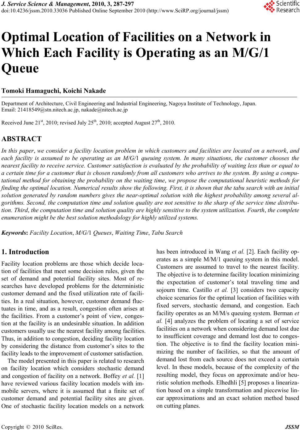J. Service Science & Management, 2010, 3, 287-297
doi:10.4236/jssm.2010.33036 Published Online September 2010 (http://www.SciRP.org/journal/jssm)
1
Optimal Location of Facilities on a Network in
Which Each Facility is Operating as an M/G/1
Queue
Tomoki Hamaguchi, Koichi Nakade
Department of Architecture, Civil Engineering and Industrial Engineering, Nagoya Institute of Technology, Japan.
Received June 21st, 2010; revised July 25th, 2010; accepted August 27th, 2010.
ABSTRACT
In this paper, we consider a facility location problem in which customers and facilities are located on a network, and
each facility is assumed to be operating as an M/G/1 queuing system. In many situations, the customer chooses the
nearest facility to receive service. Customer satisfaction is evaluated by the probability of waiting less than or equal to
a certain time for a customer that is chosen randomly from all customers who arrives to the system. By using a compu-
tational method for obtaining the probability on the waiting time, we propose the computational heuristic methods for
finding the optimal location. Numerical results show the following. First, it is shown that the tabu search with an initial
solution generated by random numbers gives the near-optimal solution with the highest probability among several al-
gorithms. Second, the computation time and solution quality are not sensitive to the sharp of the service time distribu-
tion. Third, the computation time and solution quality are highly sensitive to the system utilization. Fourth, the complete
enumeration might be the best solution methodology for highly utilized systems.
Keywords: Facility Location, M/G/1 Queues, Waiting Time, Tabu Search
1. Introduction
Facility location problems are those which decide loca-
tion of facilities that meet some decision rules, given the
set of demand and potential facility sites. Most of re-
searches have developed problems for the deterministic
customer demand and the fixed utilization rate of facili-
ties. In a real situation, however, customer demand fluc-
tuates in time, and as a result, congestion often arises at
the facilities. From a customer’s point of view, conges-
tion at the facility is an undesirable situation. In addition
customers usually use the nearest facility among facilities.
Thus, in addition to congestion, deciding facility location
by considering the distance from customer’s sites to the
facility leads to the improvement of customer satisfaction.
The model presented in this paper is related to research
on facility location which considers stochastic demand
and congestion of facility on a network. Boffey et al. [1]
have reviewed various facility location models with im-
mobile servers, where it is assumed that a finite set of
customer demand and potential facility sites are given.
One of stochastic facility location models on a network
has been introduced in Wang et al. [2]. Each facility op-
erates as a simple M/M/1 queuing system in this model.
Customers are assumed to travel to the nearest facility.
The objective is to determine facility location minimizing
the expectation of customer’s total traveling time and
sojourn time. Castillo et al. [3] considers two capacity
choice scenarios for the optimal location of facilities with
fixed servers, stochastic demand, and congestion. Each
facility operates as an M/M/s queuing system. Berman et
al. [4] analyzes the problem of locating a set of service
facilities on a network when considering demand lost due
to insufficient coverage and demand lost due to conges-
tion. The objective is to find the facility location mini-
mizing the number of facilities, so that the amount of
demand lost from each source does not exceed a certain
level. In these models, because of the complexity of the
resulting model, they focus on approximate and/or heu-
ristic solution methods. Elhedhli [5] proposes a lineariza-
tion based on a simple transformation and piecewise lin-
ear approximations and an exact solution method based
on cutting planes.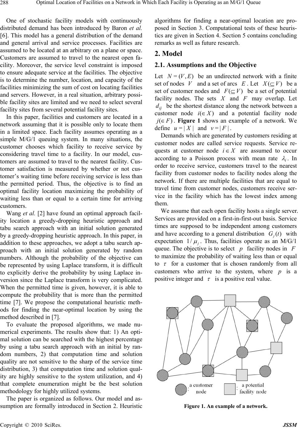

Optimal Location of Facilities on a Network in Which Each Facility is Operating as an M/G/1 Queue 288
One of stochastic facility models with continuously
distributed demand has been introduced by Baron et al.
[6]. This model has a general distribution of the demand
and general arrival and service processes. Facilities are
assumed to be located at an arbitrary on a plane or space.
Customers are assumed to travel to the nearest open fa-
cility. Moreover, the service level constraint is imposed
to ensure adequate service at the facilities. The objective
is to determine the number, location, and capacity of the
facilities minimizing the sum of cost on locating facilities
and servers. However, in a real situation, arbitrary possi-
ble facility sites are limited and we need to select several
facility sites from several potential facility sites.
In this paper, facilities and customers are located in a
network assuming that it is possible only to locate them
in a limited space. Each facility assumes operating as a
simple M/G/1 queuing system. In many situations, the
customer chooses which facility to receive service by
considering travel time to a facility. In our model, cus-
tomers are assumed to travel to the nearest facility. Cus-
tomer satisfaction is measured by whether or not cus-
tomer’s waiting time before receiving service is less than
the permitted period. Thus, the objective is to find an
optimal facility location maximizing the probability of
waiting less than or equal to a certain time for arriving
customers.
Wang et al. [2] have found an optimal approach facil-
ity location a greedy-dropping heuristic approach and
tabu search approach with an initial solution generated
by a greedy-dropping heuristic approach. In this paper, in
addition to these approaches, we adopt a tabu search ap-
proach with an initial solution generated by random
numbers. Although the probability of the objective can
be represented by using Laplace transform, it is difficult
to explicitly derive the probability by using Laplace in-
version since the Laplace transform is very complicated.
When the permitted time is given, however, it is able to
compute the probability that is more than the permitted
time [7]. We propose the computational heuristic meth-
ods for finding the near-optimal location by using the
method described in [7].
To evaluate the proposed algorithms, we made nu-
merical experiments. The results show that: 1) An opti-
mal solution can be searched with the highest percentage
by using a tabu search approach with an initial by ran-
dom numbers, 2) that computation time and solution
quality are not sensitive to the sharp of the service time
distribution, 3) that computation time and solution qual-
ity are highly sensitive to the system utilization, and 4)
that complete enumeration might be the best solution
methodology for highly utilized systems.
The paper is organized as follows. Our model and as-
sumption are formally introduced in Section 2. Heuristic
algorithms for finding a near-optimal location are pro-
posed in Section 3. Computational tests of these heuris-
tics are given in Section 4. Section 5 contains concluding
remarks as well as future research.
2. Model
2.1. Assumptions and the Objective
Let be an undirected network with a finite
set of nodes and a set of arcs . Let
=( ,)NVE
VE()
X
V be a
set of customer nodes and ()
F
V be a set of potential
facility nodes. The sets
X
and
F
may overlap. Let
ij be the shortest distance along the network between a
customer node
d
)( Xi

and a potential facility node
()Fj

. Figure 1 shows an example of a network. We
define and .
=| |uX |F|=v
Demands which are generated by customers residing at
customer nodes are called service requests. Service re-
quests at customer node are assumed to occur
according to a Poisson process with mean rate i
iX

. In
order to receive service, customers travel to the nearest
facility from customer nodes to facility nodes along the
network. If there are multiple facilities that are equal to
travel time from customer nodes, customers receive ser-
vice in the facility which has the lowest index among
them.
We assume that each open facility hosts a single server.
Services are provided on a first-in-first-out basis. Service
times are supposed to be independent among customers
and have according to a general distribution with
expectation
()
j
Gt
1/
j

. Thus, facilities operate as an M/G/1
queue. The objective is to select facility nodes in
p
F
to maximize the probability of waiting less than or equal
to

for a customer that is chosen randomly from all
customers who arrive to the system, where is a
positive integer and
p

is a positive real value.
Figure 1. An example of a network.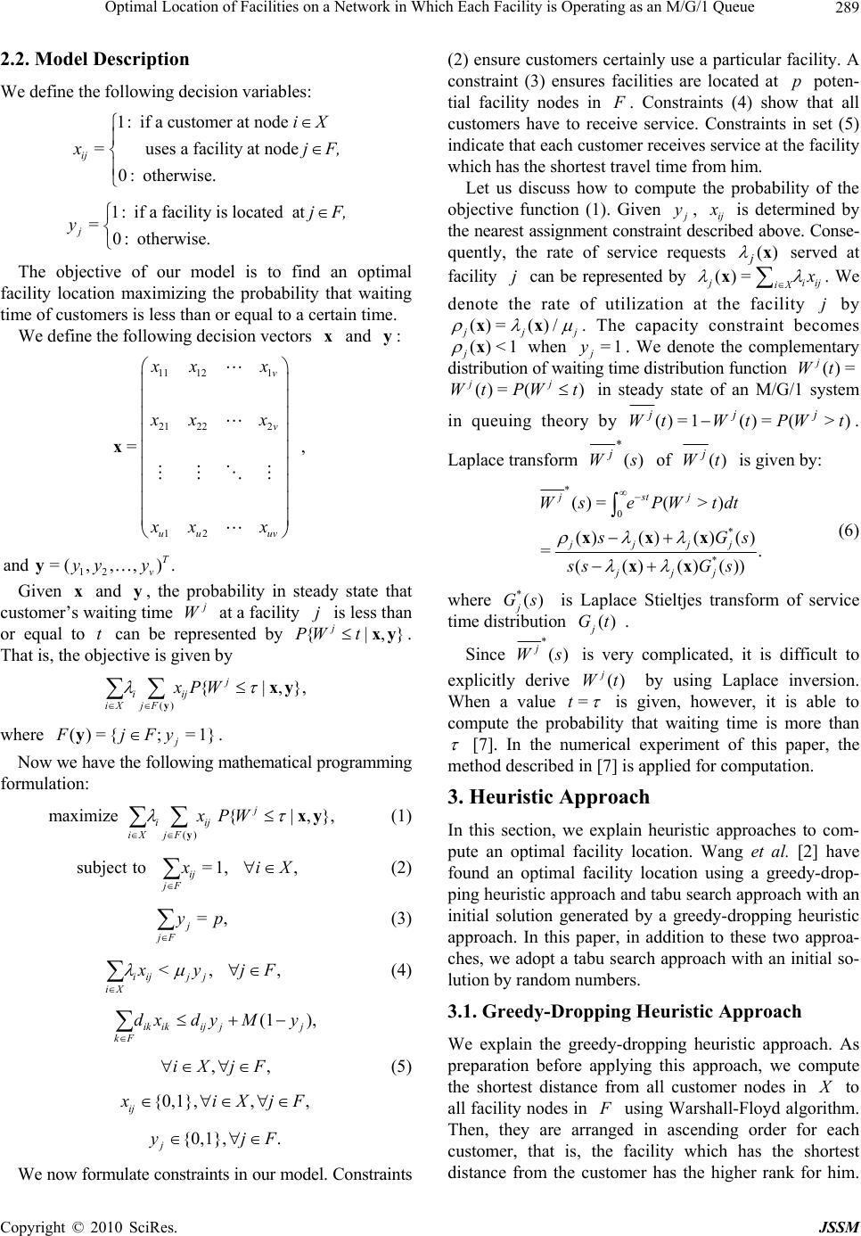

Optimal Location of Facilities on a Network in Which Each Facility is Operating as an M/G/1 Queue289
2.2. Model Description
We define the following decision variables:
1: if a customer at node
= uses a facility at node
0: otherwise.
ij
i X
x
j F,






1: if a facility is located at
=0: otherwise.
j
j F,
y



The objective of our model is to find an optimal
facility location maximizing the probability that waiting
time of customers is less than or equal to a certain time.
We define the following decision vectors and : x y
11 121
21 222
12
=
v
v
uu uv
xx x
xx x
xx x











x




,
12
and= (,,,).
T
v
yy yy
Given and , the probability in steady state that
customer’s waiting time
x y
j
W at a facility is less than
or equal to
j
t
can be represented by .
That is, the objective is given by
{|,
jtxy}
},
PW
()
{|,
j
iij
iX jF
xPW 



y
xy
where .
()={; =1}
j
FjFyy
Now we have the following mathematical programming
formulation:
()
maximize{|, },
j
iij
iX jF
xPW 



y
x
y
(1)
subjectto =1,,
ij
jF
x
iX


 (2)
=,
j
jF
yp

 (3)
<,
iijj j
iX
,
x
yjF 


 (4)
(1 ),
ik ikijjj
kF
dxdyMy



,iXjF , (5)
{0,1},, ,
ij
x
iXjF
{0,1}, .
j
yjF
We now formulate constraints in our model. Constraints
(2) ensure customers certainly use a particular facility. A
constraint (3) ensures facilities are located at poten- p
tial facility nodes in
F
. Constraints (4) show that all
customers have to receive service. Constraints in set (5)
indicate that each customer receives service at the facility
which has the shortest travel time from him.
Let us discuss how to compute the probability of the
objective function (1). Given
j
y, ij
x
is determined by
the nearest assignment constraint described above. Conse-
quently, the rate of service requests served at
)(x
j

()=
facility can be represented by
j
j
iij
iX
x



x. We
denote the rate of utilization at the facility by j
()= ()/
j
jj



xx
()<1
j
. The capacity constraint becomes

xy
()= ()
j
Wt PWt
when . We denote the complementary
distribution of waiting time distribution function
=1
j
j
()
j
Wt=

in steady state of an M/G/1 system
in queuing theory by )>(=)(1=)(tWPtWtW jj j.
Laplace transform )(
*
sW j of )(tWj is given by:
*
0
*
*
()=(> )
()()() ()
=.
(()()())
jstj
jjjj
jjj
WsePWtdt
s
Gs
ssG s






xxx
xx
(6)
where is Laplace Stieltjes transform of service
time distribution .
*()
j
Gs
()
j
Gt
Since
*
()
j
Ws is very complicated, it is difficult to
explicitly derive by using Laplace inversion.
When a value
()
j
Wt
=t

is given, however, it is able to
compute the probability that waiting time is more than

[7]. In the numerical experiment of this paper, the
method described in [7] is applied for computation.
3. Heuristic Approach
In this section, we explain heuristic approaches to com-
pute an optimal facility location. Wang et al. [2] have
found an optimal facility location using a greedy-drop-
ping heuristic approach and tabu search approach with an
initial solution generated by a greedy-dropping heuristic
approach. In this paper, in addition to these two approa-
ches, we adopt a tabu search approach with an initial so-
lution by random numbers.
3.1. Greedy-Dropping Heuristic Approach
We explain the greedy-dropping heuristic approach. As
preparation before applying this approach, we compute
the shortest distance from all customer nodes in
X
to
all facility nodes in
F
using Warshall-Floyd algorithm.
Then, they are arranged in ascending order for each
customer, that is, the facility which has the shortest
distance from the customer has the higher rank for him.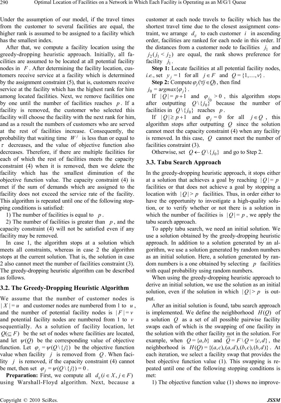

Optimal Location of Facilities on a Network in Which Each Facility is Operating as an M/G/1 Queue 290
Under the assumption of our model, if the travel times
from the customer to several facilities are equal, the
higher rank is assumed to be assigned to a facility which
has the smallest index.
After that, we compute a facility location using the
greedy-dropping heuristic approach. Initially, all fa-
cilities are assumed to be located at all potential facility
nodes in
F
. After determining the facility location, cus-
tomers receive service at a facility which is determined
by the assignment constraint (5), that is, customers receive
service at the facility which has the highest rank for him
among located facilities. Next, we remove facilities one
by one until the number of facilities reaches . If a
facility is removed, the customer who selected this
facility will choose the facility with the next rank for him,
and as a result the numbers of customers who are served
at the rest of facilities increase. Consequently, the
probability that waiting time
p
j
W is less than or equal to

decreases, and the value of objective function also
decreases. Therefore, if there are multiple facilities for
each of which the rest of facilities meets the capacity
constraint (4) when it is removed, then we delete the
facility which has the smallest diminution of the
objective function value. The capacity constraint (4) is
met if the sum of demands which are assigned to the
facility does not exceed the service rate of the facility.
This algorithm is repeated until one of the following stop-
ping conditions is satisfied:
1) The number of facilities is equal to . p
2) The number of facilities is greater than , and the
capacity constraint (4) will not be satisfied even if any
facility may be removed.
p
In case 1, the algorithm stops at a solution which
meets all constraints, whereas in case 2 the algorithm
stops at the current solution. That is, the solution in case
2 also cannot meet the number of facilities constraint (3).
The greedy-dropping heuristic algorithm can be described
as follows.
3.2. The Greedy-Dropping Heuristic Algorithm
We assume that the number of customer nodes is
||=
X
u and customer nodes are numbered from 1 to ,
and the number of potential facility nodes is
and potential facility nodes are numbered from 1 to
u
v=F||
v
sequentially. As a solution of facility location, let
be the set of nodes where facilities are located,
and let
)( FQ 
()Q

be the corresponding value of objective
function. Let =(\{})
jQj

be the objective function
value when facility is removed from . When faci- j Q
lity is removed, if the capacity constraint (4) cannot
be met, then set .
j
0=}){\(=jQ
j

Preparation: First, we compute all
using Warshall-Floyd algorithm. Next, because a
customer at each node travels to facility which has the
shortest travel time due to the closest assignment cons-
(,
ij
diXjF
traint, we arrange ij to each customer in ascending
order, facilities are ranked for each node in this order. If
the distances from a customer node to facilities 1 and
are equal, the rank shows preference for
facility .
d i
j
)<( 212 jjj
j1
Step 1: Locate facilities at all potential facility nodes,
i.e., set for all
1=
j
yFj

and . },{1,= vQ 
Step 2: Compute)Qj(
j



, then find
.
}{a=
0j
rgmaxj 
1=|| If

pQ and 0
0
j>

, this algorithm stops
after outputting Q because the number of
facilities in reaches .
}
0
j
p
{\
}{\ jQ
1||
0
If

pQ and j for all
0= 
Qj

, this
algorithm stops after outputting Q since the solution
cannot meet the capacity constraint (4) when any facility
is removed. In this case, cannot meet the number of
facilities constraint (3).
Q
Otherwise, set }{\ 0
jQQ

and go to Step 2.
3.3. Tabu Search Approach
In the greedy-dropping heuristic approach, it stops either
at a solution that achieves a goal by reaching
facilities or that does not achieve a goal by stopping a
location with facilities. Thus, in order either to
have the opportunity to investigate a high-quality solu-
tion, or to verify whether or not there is a solution in
which the number of facilities is , we apply the
tabu search approach.
pQ =||
pQ >||
pQ =||
To apply tabu search, we need an initial solution. We
use a solution obtained by the greedy-dropping heuristic
approach. In addition to a solution generated by an al-
gorithm, we use a solution generated by random numbers
as an initial solution. Here, a solution generated by ran-
dom numbers is a one obtained by selecting facilities
with equal probability using random numbers.
p
When using the greedy-dropping heuristic approach to
derive an initial solution, we use the solution as an initial
solution, even if the solution in which is out-
put.
pQ >||
After an initial solution is found, tabu search approach
is implemented. We define the neighborhood of
a solution as a set of all possible pairwise facility
swaps each of which is the swapping of one facility in
the solution with the other facility not in the solution. For
example, when and
)(QH
Q
},{= baQ},{ dc
)}, db
=\= QFQ, the
neighborhood is . At
each iteration, we select a facility swap that provides the
best objective function value (1). This swapping is re-
peated until one of the following stopping conditions is
met:
(),,(),,(),,cbdaca{(=)(QH
)
1) The objective function value (1) shows no improve-

Optimal Location of Facilities on a Network in Which Each Facility is Operating as an M/G/1 Queue291
ment at successive
K
times.
2) Even if we carry out every facility swaps in the
neighborhood, the solution cannot meet the capacity
constraint (4).
In case that we use a solution of as an initial
solution, we apply the greedy-dropping heuristic approach
to know whether the number of facilities can become
every time the facility swap is carried out. In case that a
solution meets the above stopping condition and the
number of facilities cannot be decreased, we output .
pQ >||
p
Q
Q
In case that the current solution Q is a local optimum,
it is highly likely that the solution returns to Q again by
ntinuing swaps after moving from Q to the ther
solution Q. To avoid this, we prepare for the set of
pairs of facilities called a tabu list. That is, we forbid
swapping of pairs of facilities involved in this list.
co o
To present the algorithm, we introduce the following
additional notation:
 * Q: the best solution found so far;
 L: the length of the tabu list;

K
: the maximum number of successive non-impro-
vement swaps permitted;
 ),( jiTL : the number of iterations which are
remained until facility pair ),( ji is permitted to
come up for candidates of exchange.
Note that if , pair is in the tabu list
and cannot be used in the next iterations.
Using the defined notations, we denote the neighbor-
hood of , i.e., the set of feasible facility swaps, by
. The tabu
search algorithm is as follows.
0>),( jiTL
\,: FjQi
),( ji
TL
),( ji
),( ji
0}=
Q
,{(i,)=)( TLQjQH
3.4. The Tabu Search Algorithm
Step 1: Let be the solution generated by the greedy- Q
dropping heuristic approach or the random number. Set
, and set
.
),0(=),(0,=,=
*FjijiTLkQQ 
,(,\,:),{(=)( jiTLQNjQijiQH 
)(QH
0}=)
Step 2: If is empty, stop and output .
Otherwise, swaps are tried on all pairs in , then
we search the facility swap in that meets
the capacity constraint (4) and provides the best value of
the objective function. If any facility swap in
does not meet the capacity constraint (4), this algorithm
stops after outputting . In this case, if ,
cannot meet the number of facilities constraint (3).
*
Q
)(Q
*
Q
)(QH
)
H
pQ >|
*
),( ts (QH
|
*
Q
Step 3: If )(>}){\}{( QstQ



}{\}{ st
, then set
; otherwise, set
0, *QQk  1

kk. If
, then we have performed Kk =
K
successive swaps
that do not improve the objective function value, stop
and output ; otherwise, set Q,
,
*
Q
stTLtsTL ),(=),(
}
1,0}
{\}{ stQ
),(

L= {max=),(

jiTLjiTL
),( st )(QH (), and is updated. o),(=),( rtsji  
If , go to Step 2, and if , go to Step 4. pQ =|| pQ >||
Step 4: To check whether or not the number of fa-
cilities can decrease from to , we apply the
greedy-dropping heuristic approach. When we apply the
algorithm, as an initial location of Step 1 of this algorithm,
we use the current solution . After applying the al-
gorithm, set the derived solution as , and then go to
Step 2.
|| Q
Q
p
Q
Unlike the greedy-dropping heuristic approach, the
approach with an initial solution obtained by the random
number will generate the different solution every time.
The solution obtained after the tabu search will strongly
depend on the initial solution. In the numerical experi-
ments of the next section, when we apply a tabu search
with these approaches, we repeat the tabu search with
different initial solutions five times, and output the
solution which has the best objective function among
solutions obtained after every tabu search. We can expect
that the solution obtained will be improved, since tabu
search approach is applied using a variety of initial so-
lutions.
4. Computational Results
In this section, we numerically test heuristic approaches
described in the previous section by applying various
data, and discuss the results.
4.1. Experimental Setup
In this paper, the following three experiments are con-
ducted by altering parameters.
1) the numbers of nodes
2) utilization rates and distributions
3) the number of potential facility nodes
Before starting experiments, we automatically generate
networks by using the following method. Let be the
number of total nodes in a network, and let
N
A
be the
number of total arcs in a network. Initially, we locate
nodes by using a uniform random number on a plane
region of
N
YyXx 



,00 . Next, we select two
nodes from located nodes in a random manner, and
connect them by an arc. At this time, the distance be-
tween two nodes is Euclidean, and we select
A
arcs
with avoiding duplicates. Finally, by Warshall-Floyd
algorithm, we check whether or not all nodes are
connected. If some two nodes are not connected, we
reattempt from a generation of nodes; otherwise, we
conduct a numerical experiment by using the generated
network. Figure 2 shows an example of a network
generated automatically as 100,=X100
,
=Y
by Mathematica 7.0.
200,=N
400=A
In addition, in this paper, all programs are programmed
by using C language and compiled by using Fujitsu C

Optimal Location of Facilities on a Network in Which Each Facility is Operating as an M/G/1 Queue 292
Figure 2. An example of a network using a numerical experiment.
Compiler, and executed on a PC with Intel(R) Core
(TM)2 CPU4300 1.80GHz 3GB RAM.
First, we explain approaches and parameters used in
numerical experiments. Approaches in numerical experi-
ments are as follows:
 Exhaustive search [Combination] (COMB);
 Greedy-dropping heuristic approach (GD);
 Tabu search approach with an initial solution
generated by using a greedy-dropping heuristic
approach (GD-T);
 Tabu search approach with initial solutions gene-
rated by random numbers (RAND-T).
An exhaustive search is an approach that searches an
optimal solution by computing objective values on po-
ssible all combinations. From now on, we call each
approach by the corresponding abbreviated expressions.
As discussed in the last section, the RAND-T repeat
tabu search with initial solutions generated by random

Optimal Location of Facilities on a Network in Which Each Facility is Operating as an M/G/1 Queue293
numbers five times, and then they outputs a solution that
provides the best objective function value among solu-
tions obtained by tabu search.
We explain parameters used in experiments. Based on
preliminary experimentation, the common parameters are
set as follows:
 Numerical Laplace Inversion algorithm: the number
of points conducted in the Laplace Inversion algo-
rithm simultaneously is 32;
 Tabu search algorithm: the length of a tabu list is 7;
 Tabu search algorithm: the maximum number of
successive non-improvement swaps permitted is 9.
In all experiments, we assume that each facility has the
same service rates and each customer node has the same
service request rates. In addition, we use the utilization
rates to determine the service request rates. For example,
if the number of facilities with service rate is , the
number of customer nodes is , and the utilization rate
is , the service request rate of each customer node is
set as .
1 3
10
0.6
0.18=0.6)/103)((1 
In experiment 1, we analyze the effect of the numbers
of nodes. Table 1 shows parameters used in experiment
1.
In experiment 2, we analyze the influence in the case
that utilization rates and distributions are altered. Table 2
shows parameters used in experiment 2.
In experiment 3, we analyze the influence in the case
that the number of potential facility nodes is altered. Ta-
ble 3 shows parameters used in experiment 3.
As combinations of parameters described above, ex-
periment 1 has 5 combinations. Similarly, experiment 2
has 24 combinations and experiment 3 has 4 combina-
tions. For each of 33 total combinations of parameter
values, 10 problem instances are generated, leading to a
total of 330 problem instances.
4.2. Experimental Results
Before showing the experimental results, we explain
Table 1. Parameters used in experiment 1.
Total nodes 100, 200, 300, 400, 500
Potential facility nodes 30
Customer nodes Total nodes - 300
Empty nodes 0
Facilities 5
Distribution Erlang (degree: 2)
Utilization rate 0.6
Service rate 1
Waiting time 1
Table 2. Parameters used in experiment 2.
Total nodes 500
Potential facility nodes 30
Customer nodes 470
Empty nodes 0
Facilities 5
Distribution
Exponential
Erlang (degree: 2)
Erlang (degree: 3)
Erlang (degree: 5)
Utilization rate 0.6, 0.9
Service rate 1
Waiting time 1, 3, 10
Table 3. Parameters used in experiment 3.
Potential facility nodes 20, 25, 30, 35
Customer nodes 500
Total nodes Customer nodes +
Potential facility nodes
Empty nodes 0
Facilities 5
Distribution Erlang (degree: 2)
Utilization rate 0.6
Service rate 1
Waiting time 1
following performance measures estimated by experi-
ments.
1) Optimal rate (%): a fraction of instances in which
the obtained solutions coincide with optimal solutions
obtained by the COMB.
2) Relative error (%): an average of rates obtained by
dividing absolute values of differences between the corre-
sponding optimal objective values by the COMB and
objective values by each algorithm by the former values.
3) Average computation time (seconds): average com-
putation time until the solutions are searched by each
algorithm after data of network is given.
In experiment 2, we also discuss fractions of experi-
ments that reach facilities for the solutions because
the solutions obtained by heuristics do not reach targets
on the number of facilities with high probability in some
cases.
p
4.2.1. Experiment 1
We consider the result in the case that the number of
nodes is altered. Figures 3 and 4 show average computa-

Optimal Location of Facilities on a Network in Which Each Facility is Operating as an M/G/1 Queue 294
Figure 3. Average computation time in experiment 1.
Figure 4. Optimal rates in experiment 1.
tion time and the optimal rate, respectively. Table 4
shows average values of relative errors obtained by each
algorithm. Relative errors are average values among
experiments with 100 to 500 nodes. Note that they are
almost constant on the number of nodes, and that all
solutions in this experiment have facilities. 5)(=p
From Figure 3, we can see that average computation
time of the COMB is increasing in the number of nodes.
By contrast, average computation times of the other
algorithms are not much increasing. Because the number
of potential facility nodes is set to 30, the increase of the
number of nodes implies the increase of the number of
customer nodes. Consequently, if the number of nodes
increases, the computation time necessary for determi-
ning a service facility for each customer also increases.
In the case of the COMB, because the increase of the
number of nodes has an influence on all combinations,
the running time has increased greatly. On the other hand,
because the other algorithms update solutions that meet
conditions by removing and exchanging, they can search
for the number of combinations that is much fewer than
the number of combinations in the COMB. As a result,
the increase of the number of nodes has little influence
on the running time. Because the RAND-T searches
solutions five times, that average time is longer than that
of GD.
From Figure 4, we can see that the RAND-T typically
finds the optimal solution. The fraction that it can search
the optimal solution is about 80%. It is because the tabu
search approach is conducted to a variety of directions
thanks to a diversity of initial solutions. But, the GD
cannot search optimal solutions at all. The GD-T also can
search solutions only the average of about 30%. From
Table 4, however, the relative errors of the GD is 4%,
and GD-T has smaller errors. This means that most of
cases in the GD and GD-T missed to escape from the
local optimal solution and stopped to search before
reaching the optimal solution in the tabu search.
4.2.2. Experiment 2
We show the experimental result in the case that service
time distributions and utilization rates are altered. Alth-
ough we conducted the experiment by using an exponen-
tial distribution and Erlang distributions (degree: 2,3,5),
there is not so much of differences between Erlang distri-
butions. Thus we consider the cases of an exponential
distribution and an Erlang distribution (degree: 3). Table 5
Table 4. Average of relative errors in experiment 1.
GD GD-T RAND-T
Average of relative errors0.039 0.016 0.001
Table 5. Optimal rate in the case that utilization rates and
distributions are altered.
Waiting timeGD GD-T RAND-T
1 0 0.2 0.6
3 0 0.2 0.7
Exponential: 0.6
10 0 0.3 0.9
1 0 0.2 0.2
3 0 0.3 0.1 Exponential: 0.9
10 0 0.2 0
1 0 0.2 0.8
3 0 0.2 0.8 Erlang(3): 0.6
10 0 0.3 0.5
1 0 0.2 0.1
3 0 0.3 0 Erlang(3): 0.9
10 0 0.2 0.1

Optimal Location of Facilities on a Network in Which Each Facility is Operating as an M/G/1 Queue295
shows the optimal rate in the case that utilization rates
and distributions are altered, and Table 6 shows the
average computation time.
Table 7 shows rates on searching solutions with tar-
gets on the number of facilities generated by RAND-T.
In RAND-T, we conduct tabu search with different initial
solutions five times for each instance, and we output a
solution that provides the best objective function value of
them. Thus, because we conduct experiments by using
the same parameters, Table 7 shows average of 50 total
experimental results. Table 8 shows rates of experiments
succeeding in finding solutions with targets of the
number of facilities by the other algorithms when distri-
butions and utilizations are altered.
From Table 5, for any utilization rates and distributions,
optimal rates of GD and GD-T are almost the same as in
Experiment 1. They are not influenced by

. Consequ-
ently, we can see that the distribution (Exponential or
Erlang) has almost no impact on optimal rates.
Table 6. Average computation time in the case that utiliza-
tion rates and distributions are altered.
Waiting
time GD GD-T RAND-T COMB
1 4.586 9.407 30.505 176.562
3 4.595 9.473 28.199 176.566
Exponential:
0.6
10 4.565 10.506 28.420 176.538
1 4.530 5.964 0.144 12.264
3 4.527 5.866 0.109 12.253
Exponential:
0.9
10 4.497 5.597 0.108 12.324
1 5.412 10.981 33.192 206.807
3 5.414 11.053 35.014 206.758
Erlang(3):
0.6
10 5.381 12.249 36.438 206.691
1 5.350 6.686 0.117 12.633
3 5.339 6.877 0.120 12.681
Erlang(3):
0.9
10 5.315 6.567 0.153 12.342
Table 7. Rates of experiments reaching targets of the num-
ber of facilities in solutions generated RAND-T.
Waiting time
the utilization
rate 0.6
the utilization
rate 0.9
1 0.94 0.04
3 0.88 0.04
Exponential
10 0.92 0.06
1 0.96 0.02
3 0.92 0.02 Erlang(3)
10 0.96 0.06
Table 8. Rates of experiments finding the solution that
achieves targets of the number of facilities in the case that
utilization rates and distributions are altered.
Waiting time GD GD-T
1 1.0 1.0
3 1.0 1.0
Exponential: 0.6
10 1.0 1.0
1 0.4 0.7
3 0.3 0.7 Exponential: 0.9
10 0.3 0.7
1 1.0 1.0
3 1.0 1.0 Erlang(3): 0.6
10 1.0 1.0
1 0.4 0.7
3 0.3 0.7 Erlang(3): 0.9
10 0.3 0.7
From Table 6, average computation time also are not
influenced by

. This means that the distribution have
little effect on the searching. As utilization rates are large,
however, Tables 5 and 6 show that we can hardly find
solutions even if we search from a variety of directions in
a random manner. In the case that the utilization rate is
0.6, we can almost find solutions that meet targets of the
number of facilities, but in the case that the utilization
rate is 0.9, we were hardly able to find solutions that
meet targets of the number of facilities. This is because
the number of the solutions that meet the capacity
constraint (4) decreases in the utilization rapidly. As
shown in Table 8 the same phenomenon appears in the
other algorithms. Thus, in the case that the utilization rate
is too large, it is difficult for our algorithms to search
optimal solutions or near-optimal solutions. In the case
that the utilization rate is 0.9, however, we can see that
the COMB can search optimal solutions quickly. The
computation is done quickly because the COMB skips
the computation with respect to the solution that does not
meet the capacity constraint (4) as a large majority of the
solutions cannot meet this constraint. Thus, in the case
that the utilization rate is high, the COMB is the best
algorithm in this instance.
4.2.3. Experiment 3
We consider the results in the case that the number of
potential facility nodes is altered. Targets of the number
of facilities are set to 5. Figure 5 shows optimal rates in
the case that the numbers of potential facility nodes are
altered, and Figure 6 and Table 9 show average compu-
tation time and relative errors respectively.

Optimal Location of Facilities on a Network in Which Each Facility is Operating as an M/G/1 Queue 296
Figure 5. Optimal rates in the case that potential facility
nodes are altered (A target of the number of facilities: 5).
Figure 6. Average computation time in the case that poten-
tial facility nodes are altered (A target of the number of
facilities: 5).
Table 9. Relative errors in the case that potential facility
nodes are altered (A target of the number of facilities: 5).
GD GD-T RAND-T
Potential facility nodes: 20 0.01 0.00 0.00
Potential facility nodes: 25 0.03 0.01 0.00
Potential facility nodes: 30 0.02 0.00 0.00
Potential facility nodes: 35 0.02 0.00 0.00
From Figure 5, we can see that the GD was hardly
able to search the optimal solution. The GD-T tends to
decrease optimal rates as the number of facilities increa-
ses. We can see that the optimal rates of the RAND-T are
higher than those of the other algorithm. From Table 9,
even if all algorithms increase the number of potential
facility nodes, relative errors hardly alters and they are
very small. The relative error of the RAND-T is smaller
than the other algorithm although the optimal rate is
greater. Thus, it can be concluded that the RAND-T is
the best algorithm to search an optimal facility location
in our model.
4.3. Analysis of Path Searched at the Tabu
Algorithm
The GD-T moves nearer to the optimal solution in
comparison to the solution generated by GD, but do not
reach the optimal solutions in many cases. We discuss
the reason why their approaches cannot search an op-
timal solution.
Figure 7 shows a part of the path search of the GD-T,
which searches in the order of from the facility swap 1 to
the facility swap 5. The origin of each arrow shows the
facility that is removed by exchange, and the end of the
arrow shows the facility that opens by exchange. From
Figure 7, we can see that the location returns to the first
location by the successive exchange from the facility
swap 1 to the facility swap 3. That is because this
algorithm searches toward the first solution by improving
the solution by the facility swaps 2 and 3 after it is
updated to the not-improved solution by conducting the
facility swap 1. In addition, because the algorithm cannot
exchange facilities by swap 1 in tabu list, the solution
returns to the initial location by conducting the facility
swap 5 after the solution is updated to the not-improved
solution by conducting the facility swap 4. After that,
because the swap used so far cannot be conducted, this
algorithm exchanges facilities by the other swaps in-
cluded in the neighborhood, and then this algorithm stops
by reaching the maximum number of successive non-
improvement swaps permitted. That is one of the reasons
why the algorithm sometimes accepts to update toward
the worse solution.
Figure 7. A part of the path search of the tabu search algo-
rithm.

Optimal Location of Facilities on a Network in Which Each Facility is Operating as an M/G/1 Queue 297
5. Conclusions and Future Work
This paper focuses on a facility location problem with
stochastic customer demand and congestion where cus-
tomers travel to facilities to receive services. We explain
a model that located customers and facilities on network
and provide services at each facility operating as an
M/G/1 queuing system. The objective of our model is to
search an optimal facility location maximizing the pro-
bability of waiting less than or equal to a certain time for
a customer that is chosen randomly from all customers
who arrive to the system. In order to search an optimal
location, we propose three heuristic algorithms: GD, GD-
T, and RAND-T. We conduct numerical experiments by
using these algorithms and the COMB and discuss the
properties of these algorithms.
Based on the results of numerical experiments, we can
search an optimal solution with the highest percentage by
using the RAND-T in many cases. However, in the case
that utilization rates are high, we need to search an optimal
solution by using the COMB because it is difficult for the
other three algorithms to search an optimal solution. The
tabu search approach has a property that it returns to the
first location through several facilities, which results in
stops at the local optimal solution. Although we assume
that the number of servers at each facility is set as one,
multiple servers will be considered as more realistic pro-
blems. These are also left in the future.
REFERENCES
[1] R. Boffey, R. Galvao and L. Espejo, “A Review of Con-
gestion Models in the Location of Facilities with Immo-
bile Servers,” European Journal of Operational Research,
Vol. 178, No. 3, 2007, pp. 643-662.
[2] Q. Wang, R. Batta and C. Rump, “Algorithms for a Facil-
ity Location Problem with Stochastic Customer Demand
and Immobile Servers,” Annals of Operations Research,
Vol. 111, No. 1-4, 2002, pp. 17-34.
[3] I. Castillo, A. Ingolfsson and T. Sim, “Social Optimal
Location of Facilities with Fixed Servers, Stochastic De-
mand, and Congestion,” Production and Operations Ma-
nagement, Vol. 18, No. 6, 2010, pp. 721-736.
[4] O. Berman, D. Krass and J. Wang, “Locating Service
Facilities to Reduce Lost Demand,” IIE Transactions, Vol.
38, No. 11, 2006, pp. 33-946.
[5] E. Elhedhli, “Service System Design with Immobile Serv-
ers, Stochastic Demand, and Congestion,” Manufacturing
and Service Operations Management, Vol. 8, No. 1, 2006,
pp. 92-97.
[6] O. Baron, O. Berman and D. Krass, “Facility Location
with Stochastic Demand and Constraints on Waiting
Time,” Manufacturing and Service Operations Manage-
ment, Vol. 10, No. 3, 2008, pp. 484-505.
[7] H. Tijms, “A First Course in Stochastic Models,” Wiley,
New York, 2003.