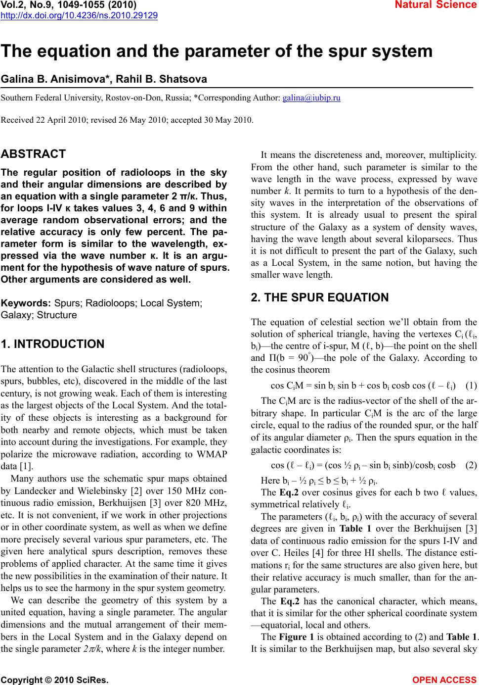
Vol.2, No.9, 1049-1055 (2010) Natural Science
http://dx.doi.org/10.4236/ns.2010.29129
The equation and the parameter of the spur system
Galina B. Anisimova*, Rahil B. Shatsova
Southern Federal University, Rostov-on-Don, Russia; *Corresponding Author:
Received 22 April 2010; revised 26 May 2010; accepted 30 May 2010.
ABSTRACT
The regular position of radioloops in the sky
and their angular dimensions are described by
an equation with a single parameter 2 π/к. Thus,
for loops I-IV к takes values 3, 4, 6 and 9 within
average random observational errors; and the
relative accuracy is only few percent. The pa-
rameter form is similar to the wavelength, ex-
pressed via the wave number к. It is an argu-
ment for the hypothesis of wave nature of spurs.
Other arguments are considered as well.
Keywords: Spurs; Radioloops; Local System;
Galaxy; Structure
1. INTRODUCTION
The attention to the Galactic shell structures (radioloops,
spurs, bubbles, etc), discovered in the middle of the last
century, is not growing weak. Each of them is interesting
as the largest objects of the Local System. And the total-
ity of these objects is interesting as a background for
both nearby and remote objects, which must be taken
into account during the investigations. For example, they
polarize the microwave radiation, according to WMAP
data [1].
Many authors use the schematic spur maps obtained
by Landecker and Wielebinsky [2] over 150 MHz con-
tinuous radio emission, Berkhuijsen [3] over 820 MHz,
etc. It is not convenient, if we work in other projections
or in other coordinate system, as well as when we define
more precisely several various spur parameters, etc. The
given here analytical spurs description, removes these
problems of applied character. At the same time it gives
the new possibilities in the examination of their nature. It
helps us to see the harmony in the spur system geometry.
We can describe the geometry of this system by a
united equation, having a single parameter. The angular
dimensions and the mutual arrangement of their mem-
bers in the Local System and in the Galaxy depend on
the single parameter 2  /k, where k is the integer number.
It means the discreteness and, moreover, multiplicity.
From the other hand, such parameter is similar to the
wave length in the wave process, expressed by wave
number k. It permits to turn to a hypothesis of the den-
sity waves in the interpretation of the observations of
this system. It is already usual to present the spiral
structure of the Galaxy as a system of density waves,
having the wave length about several kiloparsecs. Thus
it is not difficult to present the part of the Galaxy, such
as a Local System, in the same notion, but having the
smaller wave length.
2. THE SPUR EQUATION
The equation of celestial section we’ll obtain from the
solution of spherical triangle, having the vertexes Ci (ℓi,
bi)—the centre of i-spur, M (ℓ, b)—the point on the shell
and П(b = 90°)—the pole of the Galaxy. According to
the cosinus theorem
cos CiM = sin bi sin b + cos bi cosb cos (ℓ – ℓi) (1)
The CiM arc is the radius-vector of the shell of the ar-
bitrary shape. In particular CiM is the arc of the large
circle, equal to the radius of the rounded spur, or the half
of its angular diameter ρi. Then the spurs equation in the
galactic coordinates is:
cos (ℓ – ℓi) = (cos ½ ρi – sin bi sinb)/cosbi cosb (2)
Here bi – ½ ρi ≤ b ≤ bi + ½ ρi.
The Eq.2 over cosinus gives for each b two ℓ values,
symmetrical relatively ℓi.
The parameters (ℓi, bi, ρi) with the accuracy of several
degrees are given in Table 1 over the Berkhuijsen [3]
data of continuous radio emission for the spurs I-IV and
over C. Heiles [4] for three HI shells. The distance esti-
mations ri for the same structures are also given here, but
their relative accuracy is much smaller, than for the an-
gular parameters.
The Eq.2 has the canonical character, which means,
that it is similar for the other spherical coordinate system
—equatorial, local and others.
The Figure 1 is obtained according to (2) and Table 1.
It is similar to the Berkhuijsen map, but also several sky

G. B. Anisimova et al. / Natural Science 2 (2010) 1049-1055
1050
Table 1. The shell parameters over the radio data.
i Shells ℓi b
i ρi r i (pc) кi
1 I 329 ± 1.5 17.5 ± 3 116 ± 4 130 ± 75 3 = 1 × 3
2 II 100 ± 2 –32,5 ± 3 91 ± 4 110 ± 40 4 = (1 – ¼)-1 × 3
3 III 124 ± 2 15.5 ± 3 65 ± 3 150 ± 50 6 = 2 × 3
4 IV 315 ± 3 48.5 ± 1 40 ± 2 250 ± 90 9 = 3 × 3
5 Gum Neb 258 ± 2 –2 ± 1 36 415
10 = (1 – 1/10)-1 × 9
6 Eridan 205 –19 40 440 9 = 3 × 3
7 Orion Neb 209 –19 40 440 9 = 3 × 3
Z
1
GB
X
S
S
Z
3
E
E
GB
Z
2


MW 
 
П
1
П
3
II
III
I
IV
Gum
Eri
Ori
MW
-90
-60
-30
0
30
60
90
-180-150-120 -90-60-300306090120 150 180
l
b
Figure 1. The analytical map of the radioloop system in the
galactic coordinates. The circles of local and galactic triedrs
and their poles Z1,Z2,Z3 and П1, П2, П3 are shown.
orienteers, mentioned below, are added.
3. THE SPURS SYSTEM
The similarity in the astronomical sense, the spherical
shape of large objects and mutual proximity (ri  0,5 kpc)
permit us to combine all these spurs into the united sys-
tem (or the subsystem of Local system). Let us join to
these features several else, following from the observa-
tions and showing the peculiarities of the Eq.2.
3.1. The Angular Loop Diameters
The angular loop diameters i within average random ob-
servational errors over the Table 1 data can be rounded
up to
ρi = 2π/кi (3)
where кi is the integer number: 3, 4, 6, 9, 10. Moreover,
for the majority of the shells these numbers are divisible
to 3. To have no exclusions, we may perform (3) for
Loop II, as a combination
ρII = 2π/4 = 2π/1×3 – 2π/4×3, (3a)
here both members have the denominators, divisible by
the typical number k0 = 3. For Gum Neb, having k = 9 or
10, the second variant may perform the combination
10 = (3 + 1/3) × 3= (1-1/10)-1 × 9. (3b)
The Local bubble also is a part of spurs system [5]. As
the Sun is inside this bubble, its кi = 1.
If the linear radiuses of the loops from Table 1 are
almost the same (about 100 pc), as admit Berkhuijsen [3]
and other authors, then (3) means the dependence for the
distances r:
ri/rj = (sin ρj/2)/(sin ρi/2) ≈ sin (π/кj)/sin (π/кi) (4)
The r estimations and their large mean square errors
do not exclude it. For instance, the nearby Loop I and
about 2,5-3 times more remote Gum Neb and Eridan
Loop.
3.2. The Loops Arrangement Relatively the
Poles
We have shown in [6] and [7] that the centers of ra-
dioloops I-IV are situated on the small circle S`, parallel
to the equator S (Figure 1), having the common pole Z1.
The large part of spur areas is arranged at the sky zone
between S and S`, that had formed its name “the Spurs
Belt”.
Z1 is situated near or even on the intersection of the
circles of “the Dolidze net” [8], describing the Local sys-
tem. This net includes the belts – Gould, Vaucouleurs–
Dolidze, the perpendicular to them and others, connected
with the spurs. The Gould belt (GB) (Figure 1) passes
through the nucleuses of Loop I and Eri-Ori complex,
through the intersection of Loops II and III, almost
touches the Gum Neb. ┴GB circle divides the spurs sys-
tem into two groups: (the Loops I, IV, Gum Neb) and
(the Loops II, III, Eri-Ori), and it touches the Loop II
shell and recently discovered Loop VI [9].
The circles S, GB and ┴GB form the local triedr (Z1,
Z2, Z3). The coordinates of triedr poles we can obtain
over the coordinates of I-IV centres from Table 1, using
(1) for M = Z1. The approximate ℓZ1we can obtain mak-
ing equal the right parts of

G. B. Anisimova et al. / Natural Science 2 (2010) 1049-1055
105
1051
cos Z1Ci = sin bz1 sin bi + cos bz1 cosbi cos(ℓi –ℓz1) (5)
for Loops I and III and taking into account bI ≈ bIII. Us-
ing Loops II and III and the obtained ℓZ1, we derive bZ1.
So, in accuracy of several degrees ℓZ1 = 47˚, bZ1 = 21˚.
We can obtain Z2 (315˚, 7˚) and Z3 (207˚, 68˚), using
(5) and the circles S and ┴GB parameters [7] for or-
thogonal directions of axis of one of the triedrs.
Let us note, that the inclination of Z3 axis and large
circle S to the Galactic plane (MW) is about 2π/5, and
bZ1 ≈ π/2 – 2π/5.
p1, p2 and p3—the polar distances of the spur centres
Ci from the poles of Z1 - triedrs are given in the Table 2
for four main spurs confirm the Z1 coordinates and its
equidistant position, that we obtained firstly in [6] by the
other method.
where p1  p1(i) (analogous for p2 and p3)
The concrete p1 differ from the mean <p1> = 74˚ ≈
2π/5 within average random observational errors of Ci
coordinates. It is interesting that p1 ≈ 2 × 2π/5 for Gum
Neb, and p1 ≈ π/2 + 2π/5 for Eri-Ori complex, that
means that each p1 corresponds to (3) or their combina-
tions when к = 5. But here they are related to Z1 pole
and .radius Z1Ci, but not the diameter.
Table 2 also shows the interesting combinations of
spurs localization relative the other axes of Local triedr
(Z2 and Z3), symmetrical relative the opposite poles,
similar at the same distances. And the relations between
all system members, that is:
p2,3 (II) + p2,3 (IV) ≈ π, in the plane S`
p3(I) ≈ p3 (III) ≈ p3 (Gum) ≈ p3 (II) - p3 (IV)  2π/5
p2 (III) – p2 (II) ≈ p2 (Gum) – p2 (IV) ≈
p2 (Ori) – π/2 = p2 (I) ≈ π/2 – 2π/5 (6)
p3 (Eri) = p3 (Ori) ≈ π/2, etc
Table 2. The polar distances of loop centres from the triedr
poles.
Local triedr Z1Z2Z3 Galactic triedr Π1Π2Π3
i Loop
p1 p2 p3 p1` p2` p3`
1 I 74 17 75 72,5 126 41
2 II 73 139 126 122,5 33 93
3 III 72 155 73 74,5 31 116
4 IV 76 41 52 41,5 121 66
5 Gum 145 57 78 92 161 109
6 Eri 159 111 87 109 107 154
7 Ori 168 107 87 109 111 151
where p1  p1(i) (analogous for p2 and p3)
The second part of Table 2 gives the polar distances
p` from the poles of the Galactic triedr: p1` from Π1 ≡ Π
(b = 90˚), p2` from Π2 ≡ (MW, Λ) at (ℓ = 97˚, b = 0) and
p3` from Π3 ≡ (MW, ┴MW) at (ℓ = 7˚, b = 0), (Figure 1).
Here Λ is the Polar Ring of the Galaxy, intersecting
MW at the longitudes ℓ = 97˚ and 277˚. Both bright and
faint stars, as well as the galaxies of the Local group [10]
and the Virgo supergalaxy [11] are concentrated to the Λ
circle. And relative to the shells: Λ touches the loops I,
III and Gum, passes through the centre of Loop II. The
┴MW circle, orthogonal both MW, and Λ, intersects the
most active Loop I region—the North Polar Spur and
touches the Eridan shell (Figure 1).
The Loops I and III centres have almost the same p1`
≈ 2π/5; the same as p1 and p3, according to Table 2. Thus,
the Loops I and III centres are equidistant from the
northern poles Π1, Z1 и Z
3, are symmetrically arranged
relative the Π1, Z1 plane. The triangles CI Π1Z1 and CIII
Π1 Z
1 have almost equal sides ≈ 2π/5. The Eri and Ori
centres are at the same distance from the southern poles
Π1, Π2 and Z2, and Gum from Π3. There are interesting
combinations also in p2` and p3`, as well as between
them and p1`, including к = 2, 3, 4, 5, 12:
p2` (II) ≈ p2` (III) ≈ p2` (I) - π/2 ≈ π/6
p1` (Gum) ≈ p3` (II) ≈ π/2
p3` (Ori, Eri) ≈ π - π/6 (7)
p2` (I) ≈ p2` (IV) ≈ p1` (II) ≈ 2π/3
p2` (Gum) ≈ π/2 + 2π/5
p3` (III) ≈ π - p3` (IV)
The numerous relations inside each triedr and between
them for all shells show the unity and the harmony of
this system itself as well as the relations of the triedrs
presenting the Galaxy and Local system.
3.3. The Mutual Spurs Arrangement
The position of Loops I-IV centres on S’ circle (p1 ≈
2π/5) is not random. One can see this from (6) и (7). The
differences of the azimuthal coordinates Δs in the Local
System (s, p) show this more concentrative. The angle s
can be obtained from the triangle Z1Π1Ci
sin p1 sin (s - sΠ) = cosb sin (ℓ - ℓZ1) (8),
here sΠ is the angle for the northern pole of the Galaxy.
If s begins from the Loop I centre (sI = 0), then sΠ =
285˚.
The angular distances between the centres of the
neighbouring loops can be rounded in each of two
groups up to
sIII – sII = 56˚ ≈ 2π/6 = π/2 – π/6
sI – sIV = 34˚ ≈ π/6 (9)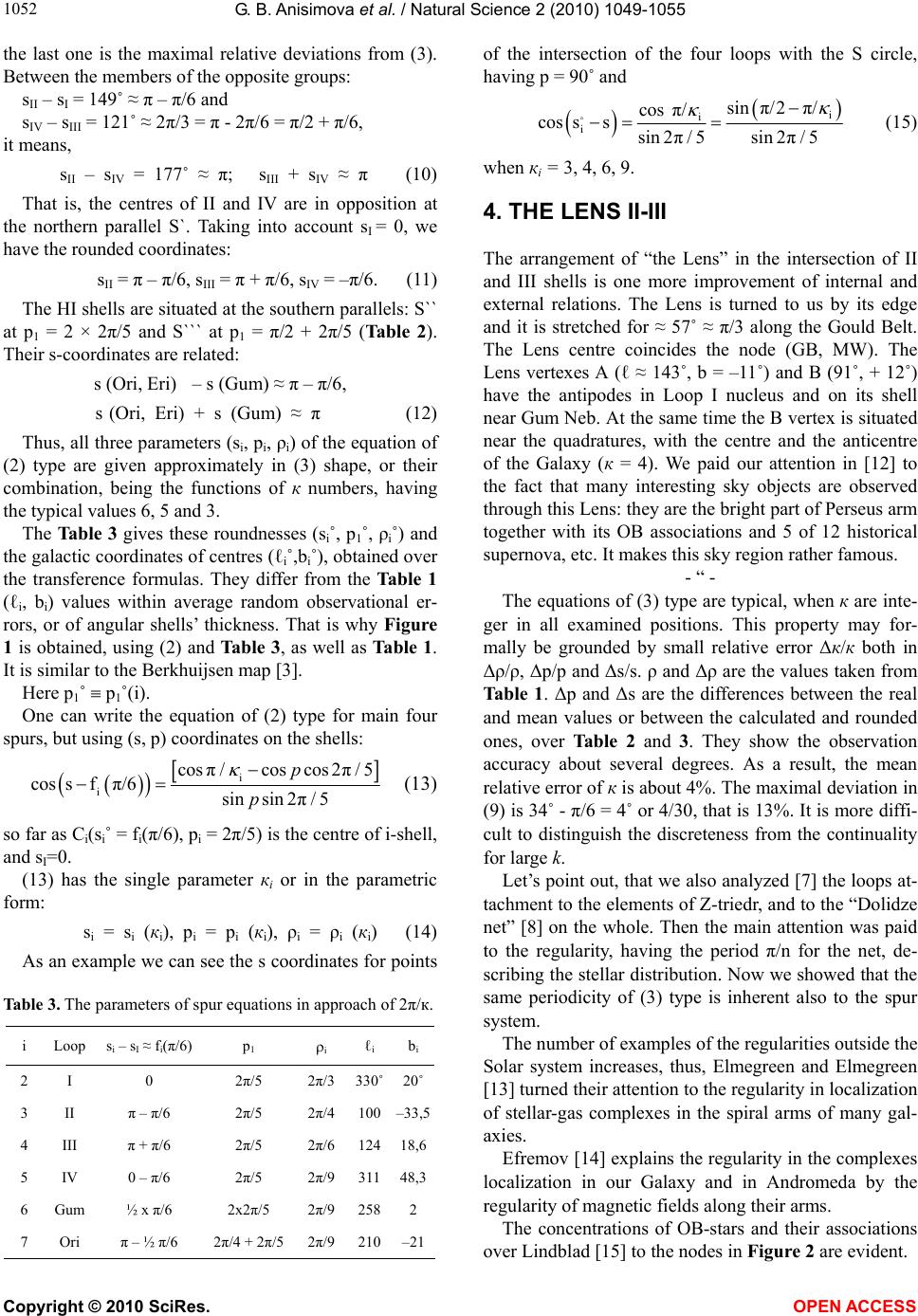

G. B. Anisimova et al. / Natural Science 2 (2010) 1049-1055
1052
the last one is the maximal relative deviations from (3).
Between the members of the opposite groups:
sII – sI = 149˚ ≈ π – π/6 and
sIV – sIII = 121˚ ≈ 2π/3 = π - 2π/6 = π/2 + π/6,
it means,
sII – sIV = 177˚ ≈ π; sIII + sIV ≈ π (10)
That is, the centres of II and IV are in opposition at
the northern parallel S`. Taking into account sI = 0, we
have the rounded coordinates:
sII = π – π/6, sIII = π + π/6, sIV = –π/6. (11)
The HI shells are situated at the southern parallels: S``
at p1 = 2 × 2π/5 and S``` at p1 = π/2 + 2π/5 (Table 2).
Their s-coordinates are related:
s (Ori, Eri) – s (Gum) ≈ π – π/6,
s (Ori, Eri) + s (Gum) ≈ π (12)
Thus, all three parameters (si, pi, ρi) of the equation of
(2) type are given approximately in (3) shape, or their
combination, being the functions of к numbers, having
the typical values 6, 5 and 3.
The Table 3 gives these roundnesses (si˚, p1˚, ρi˚) and
the galactic coordinates of centres (ℓi˚,bi˚), obtained over
the transference formulas. They differ from the Table 1
(ℓi, bi) values within average random observational er-
rors, or of angular shells’ thickness. That is why Figure
1 is obtained, using (2) and Table 3, as well as Table 1.
It is similar to the Berkhuijsen map [3].
Here p1˚  p1˚(i).
One can write the equation of (2) type for main four
spurs, but using (s, p) coordinates on the shells:
 


i
i
cos π/coscos2π/5
cos sfπ/6 sinsin 2π/5
p
p
 
 (13)
so far as Ci(si˚ = fi(π/6), pi = 2π/5) is the centre of i-shell,
and sI=0.
(13) has the single parameter кi or in the parametric
form:
si = si (кi), pi = pi (кi), ρi = ρi (кi) (14)
As an example we can see the s coordinates for points
Table 3. The parameters of spur equations in approach of 2π/к.
i Loop si – sI ≈ fi(π/6) p1 i ℓi b
i
2 I 0 2π/5 2π/3 330˚20˚
3 II π – π/6 2π/5 2π/4 100–33,5
4 III π + π/6 2π/5 2π/6 12418,6
5 IV 0 – π/6 2π/5 2π/9 31148,3
6 Gum ½ x π/6 2x2π/5 2π/9 2582
7 Ori π – ½ π/6 2π/4 + 2π/5 2π/9 210–21
of the intersection of the four loops with the S circle,
having p = 90˚ and


i
i
i
sin π/2 π/
cos π/
cos sssin 2π/5 sin2π/5



 
。 (15)
when кi = 3, 4, 6, 9.
4. THE LENS II-III
The arrangement of “the Lens” in the intersection of II
and III shells is one more improvement of internal and
external relations. The Lens is turned to us by its edge
and it is stretched for ≈ 57˚ ≈ π/3 along the Gould Belt.
The Lens centre coincides the node (GB, MW). The
Lens vertexes А (ℓ ≈ 143˚, b = –11˚) and В (91˚, + 12˚)
have the antipodes in Loop I nucleus and on its shell
near Gum Neb. At the same time the B vertex is situated
near the quadratures, with the centre and the anticentre
of the Galaxy (к = 4). We paid our attention in [12] to
the fact that many interesting sky objects are observed
through this Lens: they are the bright part of Perseus arm
together with its OB associations and 5 of 12 historical
supernova, etc. It makes this sky region rather famous.
- “ -
The equations of (3) type are typical, when к are inte-
ger in all examined positions. This property may for-
mally be grounded by small relative error Δк/к both in
Δρ/ρ, Δр/р and Δs/s. ρ and Δρ are the values taken from
Table 1. Δp and Δs are the differences between the real
and mean values or between the calculated and rounded
ones, over Table 2 and 3. They show the observation
accuracy about several degrees. As a result, the mean
relative error of к is about 4%. The maximal deviation in
(9) is 34˚ - π/6 = 4˚ or 4/30, that is 13%. It is more diffi-
cult to distinguish the discreteness from the continuality
for large k.
Let’s point out, that we also analyzed [7] the loops at-
tachment to the elements of Z-triedr, and to the “Dolidze
net” [8] on the whole. Then the main attention was paid
to the regularity, having the period π/n for the net, de-
scribing the stellar distribution. Now we showed that the
same periodicity of (3) type is inherent also to the spur
system.
The number of examples of the regularities outside the
Solar system increases, thus, Elmegreen and Elmegreen
[13] turned their attention to the regularity in localization
of stellar-gas complexes in the spiral arms of many gal-
axies.
Efremov [14] explains the regularity in the complexes
localization in our Galaxy and in Andromeda by the
regularity of magnetic fields along their arms.
The concentrations of OB-stars and their associations
over Lindblad [15] to the nodes in Figure 2 are evident.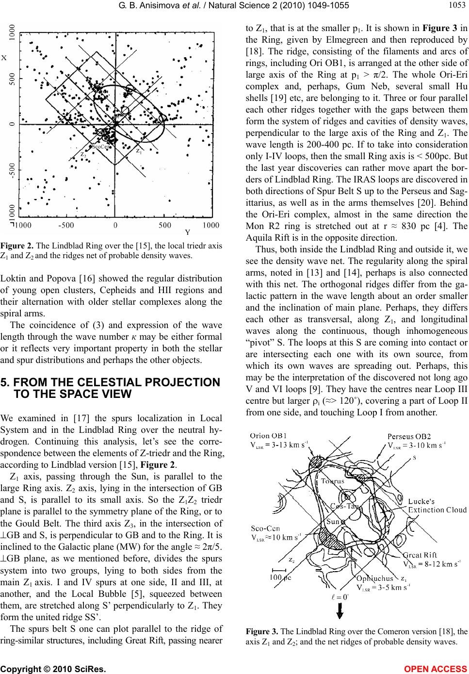

G. B. Anisimova et al. / Natural Science 2 (2010) 1049-1055
105
1053
Figure 2. The Lindblad Ring over the [15], the local triedr axis
Z1 and Z2 and the ridges net of probable density waves.
Loktin and Popova [16] showed the regular distribution
of young open clusters, Cepheids and HII regions and
their alternation with older stellar complexes along the
spiral arms.
The coincidence of (3) and expression of the wave
length through the wave number к may be either formal
or it reflects very important property in both the stellar
and spur distributions and perhaps the other objects.
5. FROM THE CELESTIAL PROJECTION
TO THE SPACE VIEW
We examined in [17] the spurs localization in Local
System and in the Lindblad Ring over the neutral hy-
drogen. Continuing this analysis, let’s see the corre-
spondence between the elements of Z-triedr and the Ring,
according to Lindblad version [15], Figure 2.
Z1 axis, passing through the Sun, is parallel to the
large Ring axis. Z2 axis, lying in the intersection of GB
and S, is parallel to its small axis. So the Z1Z2 triedr
plane is parallel to the symmetry plane of the Ring, or to
the Gould Belt. The third axis Z3, in the intersection of
GB and S, is perpendicular to GB and to the Ring. It is
inclined to the Galactic plane (MW) for the angle ≈ 2π/5.
GB plane, as we mentioned before, divides the spurs
system into two groups, lying to both sides from the
main Z1 axis. I and IV spurs at one side, II and III, at
another, and the Local Bubble [5], squeezed between
them, are stretched along S’ perpendicularly to Z1. They
form the united ridge SS’.
The spurs belt S one can plot parallel to the ridge of
ring-similar structures, including Great Rift, passing nearer
to Z1, that is at the smaller p1. It is shown in Figure 3 in
the Ring, given by Elmegreen and then reproduced by
[18]. The ridge, consisting of the filaments and arcs of
rings, including Ori OB1, is arranged at the other side of
large axis of the Ring at p1 > π/2. The whole Ori-Eri
complex and, perhaps, Gum Neb, several small Hu
shells [19] etc, are belonging to it. Three or four parallel
each other ridges together with the gaps between them
form the system of ridges and cavities of density waves,
perpendicular to the large axis of the Ring and Z1. The
wave length is 200-400 pc. If to take into consideration
only I-IV loops, then the small Ring axis is < 500pc. But
the last year discoveries can rather move apart the bor-
ders of Lindblad Ring. The IRAS loops are discovered in
both directions of Spur Belt S up to the Perseus and Sag-
ittarius, as well as in the arms themselves [20]. Behind
the Ori-Eri complex, almost in the same direction the
Mon R2 ring is stretched out at r ≈ 830 pc [4]. The
Aquila Rift is in the opposite direction.
Thus, both inside the Lindblad Ring and outside it, we
see the density wave net. The regularity along the spiral
arms, noted in [13] and [14], perhaps is also connected
with this net. The orthogonal ridges differ from the ga-
lactic pattern in the wave length about an order smaller
and the inclination of main plane. Perhaps, they differs
each other as transversal, along Z1, and longitudinal
waves along the continuous, though inhomogeneous
“pivot” S. The loops at this S are coming into contact or
are intersecting each one with its own source, from
which its own waves are spreading out. Perhaps, this
may be the interpretation of the discovered not long ago
V and VI loops [9]. They have the centres near Loop III
centre but larger i (≈> 120˚), covering a part of Loop II
from one side, and touching Loop I from another.
0



Figure 3. The Lindblad Ring over the Comeron version [18], the
axis Z1 and Z2; and the net ridges of probable density waves.

G. B. Anisimova et al. / Natural Science 2 (2010) 1049-1055
1054
And the kinematic aspect must be examined, as well.
We paid attention in [6] to the coincidence of the coor-
dinates of Solar motion apex and the Pole of Spur sys-
tem Z1. The basic motion apex (ℓA = 45˚, bA = 24˚) coin-
cides with Z1 in accuracy of several degrees. And (3)
takes place relatively the Pole Z1 isn’t it? The Sun moves
parallel to the large axis of the Lindblad Ring, that is
along the spreading of possible transversal waves. The
same is preferential motion of the majority of stars and
moving clusters in the Solar vicinity [21]. The Koval-
sky-Kapteyn figures show the same [6].
We think that these facts themselves show the exis-
tence of the wave process.
6. CONCLUSIONS
The map of spurs system (Figure 1), obtained by the
analytic method, is identical to the Berkhuijsen map, ob-
tained over the radio isophots. The spurs equation has 3
parameters: the angular diameters and their centre coor-
dinates. The spurs system is so harmonious, that assume
a number of empiric correlations between the elements
of all its members. Both the parameters of each spur and
the spur system in approach can be described by the sin-
gle parameter of 2π/к type, where к—the integer num-
bers, many of them are divisible to ко = 3. The ra-
dioloops are the largest objects of Local System. But the
statistics is small, as they are not numerous. So, the indi-
vidual observed data and their accuracy are so important.
If the discreteness and multiplicity of 2π/к parameter is
considered as a hypothesis, then it has very good accu-
racy (several percents), in comparison to many other
astronomical hypotheses.
1) The equation, describing the spurs system geometry,
and the analysis of its parameters gives the possibility to
see its structure and regular nature from the other side. It
permits to create new perspective hypotheses.
The simplified one-parametrical model may be a stage,
preceding and approaching the creation of theory of
structure – dynamics – evolution of spurs system as a
part of the Local System. The harmony of this system
shows the united and non-random formation process
(instead of, for example, the incidental supernova burst).
The type of 2π/к parameter (if it is not formal) may be a
hint to the wave nature of spur system.
2) Perhaps, the spur groups form the ridges, orthogo-
nal to the spiral arms, and together they form the wave
dense net. Thus one ridge S contains the main spurs I-IV,
Local Bubble and several IRAS loops. The other ridges
contain the Ori-Eri complex and Gum Neb. But these
and several other arguments can not immediately solve
the net problem.
3) The analytical approach can be useful in finding
new members of spur system and in solving other prob-
lems.
REFERENCES
[1] Page, L., Hinshaw, G., Komatsu, E., et al. (2007) Three
year wilkinson microwave anisotropy probe observa-
tions: Polarization analysis. The Astrophysical Journal
Supplement Series, 170(2), 335-376.
[2] Landecker, T.L. and Wielebinski, R. (1970) The galactic
metre wave radiation. Australian Journal of Physics.
Astrophysical Supplement, 16, 1-20.
[3] Berkhuijsen, E.M. (1973) Galactic continuum loops and
the diameter-surface brightness relation for supernova
remnants. Astronomy & Astrophysics, 24, 143-147.
[4] Heiles, C. (1998) Whence the local bubble, gum, orion?
Astrophysical Journal, 498, 689-703.
[5] Lallement, R., Welsh, B.Y., Vergely J.L., et al. (2003) 3D
mapping of the dense interstellar gas around the local
bubble. Astronomy & Astrophysics, 411(3), 447-464.
[6] Shatsova, R.B. and Anisimova, G.B. (2002) The spur
system in ecliptic coordinates. Astrophysics, 45(4),
535-546.
[7] Shatsova, R.B. and Anisimova, G.B. (2003) The local
system harmony. Astrophysics, 46(2) , 319-329.
[8] Dolidze, M.V. (1980) Peculiarities of local spiral arm
features of the Galaxy. Letters to Astronomical Journal, 6,
745-749
[9] Borka, V., Milogradov-Turin, J. and Uroševic, D. (2008)
The brightness of the galactic radio loops at 1420 MHz:
some indications for the existence of loops V and VI. As-
tronomische Nachrichten, 329(4), 397-402.
[10] Drosdovsky, I. (2007) The local group of galaxies.
http://www.astronet.ru/db/msg/1169715
[11] De Vaucouleurs, G., Val, A. and Corwin, H.G. (1976)
Second reference catalogue of bright galaxies, Austin,
London.
[12] Shatsova, R.B. and Anisimova, G.B. (2008) The large sky
Lens. Odessa Astronomical Publications, 21, 106-107.
[13] Elmegreen, B.G. and Elmegreen, D.M. (1983) Monthly
notices of the royal astronomical society, 203, 31.
[14] Efremov, Y.N. (2004) Stellar complexes and starburst
cumps. Proceedings of Astrophysics and Cosmology after
Gamow, Odessa, 90.
[15] Lindblad, P.O. (2000) On the rotation of Gould Belt.
Astronomy & Astrophysics, 363(1), 154-158.
[16] Loktin, A.V. and Popova M.E. (2007) The vave-
let-smoothed distribution of young stellar objects in the
galactic plane. Astronomicheskiĭ Zhurnal, in Russian,
84(5), 409-417.
[17] Shatsova, R.B. and Anisimova, G.B. (1997) The dy-
namical scheme of local system. In: Agekian, T.A., Mul-
lari, A.A. and Orlov, V.V., Eds., Structure and Evolution
of Stellar Systems, St. Peterburg University Press,
184-188.
[18] Comeron, F. (1997) The Gould Belt. In: Agekian, T.A.,
Mullari, A.A. and Orlov, V.V., Eds., Structure and Evolu-
tion of Stellar Systems, St. Peterburg University Press,
161-173.
[19] Hu, E. (1981) High latitude HI shells in the Galaxy.I.
Astrophysical Journal, 248, 119-127.

G. B. Anisimova et al. / Natural Science 2 (2010) 1049-1055
105
1055
[20] Könyvers, V., Kiss, Cs., Moor, A., et al. (2007) Cata-
logue of far-infra-red loops in the Galaxy. Astronomy and
Astrophysics, 463(3), 1227-1234.
[21] Popovic, G.M., Ninkovic, S. and Pavlovic, R. (1997) A
kinematical approach to the separation of moving-cluster
members. In: Agekian, T.A., Mullari, A.A. and Orlov,
V.V., Eds., Structure and Evolution of Stellar Systems, St.
Peterburg University Press, 108-113.