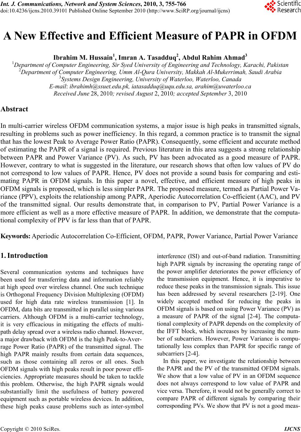Int. J. Communications, Network and System Sciences, 2010, 3, 755-766
doi:10.4236/ijcns.2010.39101 Published Online September 2010 (http://www.SciRP.org/journal/ijcns)
A New Effective and Efficient Measure of PAPR in OFDM
Ibrahim M. Hussain1, Imran A. Tasadduq2, Abdul Rahim Ahmad3
1Department of Computer Engineering, Sir Syed University of Engineering and Technology, Karachi, Pakistan
2Department of Computer Engineering, Umm Al-Qura University, Makkah Al-Mukerrimah, Saudi Arabia
3Systems Design Engineering, University of Waterloo, Waterloo, Canada
Received June 28, 2010; revised August 2, 2010; accepted September 3, 2010
Abstract
In multi-carrier wireless OFDM communication systems, a major issue is high peaks in transmitted signals,
resulting in problems such as power inefficiency. In this regard, a common practice is to transmit the signal
that has the lowest Peak to Average Power Ratio (PAPR). Consequently, some efficient and accurate method
of estimating the PAPR of a signal is required. Previous literature in this area suggests a strong relationship
between PAPR and Power Variance (PV). As such, PV has been advocated as a good measure of PAPR.
However, contrary to what is suggested in the literature, our research shows that often low values of PV do
not correspond to low values of PAPR. Hence, PV does not provide a sound basis for comparing and esti-
mating PAPR in OFDM signals. In this paper a novel, effective, and efficient measure of high peaks in
OFDM signals is proposed, which is less simpler PAPR. The proposed measure, termed as Partial Power Va-
riance (PPV), exploits the relationship among PAPR, Aperiodic Autocorrelation Co-efficient (AAC), and PV
of the transmitted signal. Our results demonstrate that, in comparison to PV, Partial Power Variance is a
more efficient as well as a more effective measure of PAPR. In addition, we demonstrate that the computa-
tional complexity of PPV is far less than that of PAPR.
Keywords: Aperiodic Autocorrelation Co-Efficient, OFDM, PAPR, Power Variance, Partial Power Variance
1. Introduction
Several communication systems and techniques have
been used for transferring data and information reliably
at high speed over wireless channel. One such technique
is Orthogonal Frequency Division Multiplexing (OFDM)
used for high data rate wireless transmission [1]. In
OFDM, data bits are transmitted in parallel using various
carriers. Although OFDM is a multi-carrier technology,
it is very efficacious in mitigating the effects of multi-
path delay spread over a wireless radio channel. However,
a major drawback with OFDM is the high Peak-to-Aver-
rage Power Ratio (PAPR) of the transmitted signal. The
high PAPR mainly results from certain data sequences,
such as those containing all zeros or all ones. Such
OFDM signals with high peaks result in poor power effi-
ciencies. Appropriate measures should be taken to tackle
this problem. Otherwise, the high PAPR signals would
substantially limit the usefulness of battery powered
equipment such as portable wireless devices. In addition,
these high peaks cause problems such as inter-symbol
interference (ISI) and out-of-band radiation. Transmitting
high PAPR signals by increasing the operating range of
the power amplifier deteriorates the power efficiency of
the transmission equipment. Hence, it is imperative to
reduce these peaks in the transmission signals. This issue
has been addressed by several researchers [2-19]. One
widely accepted method for reducing the peaks in
OFDM signals is based on using Power Variance (PV) as
a measure of PAPR of the signal [2-4]. The computa-
tional complexity of PAPR depends on the complexity of
the IFFT block, which increases by increasing the num-
ber of subcarriers. However, Power Variance is compu-
tationally less complex than PAPR for specific range of
subcarriers [2-4].
In this paper, we investigate the relationship between
the PAPR and the PV of the transmitted OFDM signals.
We show that a low value of PV in an OFDM sequence
does not always correspond to low value of PAPR and
vice versa. Therefore, it would not be generally correct to
compare PAPR of different signals by comparing their
corresponding PVs. We show that PV is not a good meas-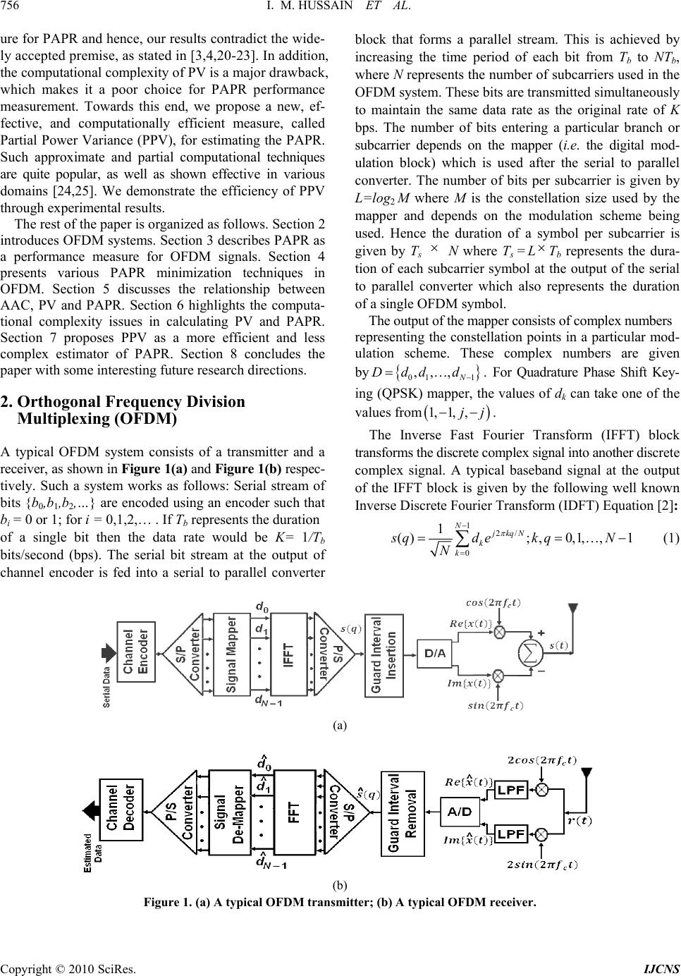

756 I. M. HUSSAIN ET AL.
ure for PAPR and hence, our results contradict the wide-
ly accepted premise, as stated in [3,4,20-23]. In addition,
the computational complexity of PV is a major drawback,
which makes it a poor choice for PAPR performance
measurement. Towards this end, we propose a new, ef-
fective, and computationally efficient measure, called
Partial Power Variance (PPV), for estimating the PAPR.
Such approximate and partial computational techniques
are quite popular, as well as shown effective in various
domains [24,25]. We demonstrate the efficiency of PPV
through experimental results.
The rest of the paper is organized as follows. Section 2
introduces OFDM systems. Section 3 describes PAPR as
a performance measure for OFDM signals. Section 4
presents various PAPR minimization techniques in
OFDM. Section 5 discusses the relationship between
AAC, PV and PAPR. Section 6 highlights the computa-
tional complexity issues in calculating PV and PAPR.
Section 7 proposes PPV as a more efficient and less
complex estimator of PAPR. Section 8 concludes the
paper with some interesting future research directions.
2. Orthogonal Frequency Division
Multiplexing (OFDM)
A typical OFDM system consists of a transmitter and a
receiver, as shown in Figure 1(a) and Figure 1(b) respec-
tively. Such a system works as follows: Serial stream of
bits {b0,b1,b2,…} are encoded using an encoder such that
bi = 0 or 1; for i = 0,1,2,… . If Tb represents the duration
of a single bit then the data rate would be K= 1/Tb
bits/second (bps). The serial bit stream at the output of
channel encoder is fed into a serial to parallel converter
block that forms a parallel stream. This is achieved by
increasing the time period of each bit from Tb to NTb,
where N represents the number of subcarriers used in the
OFDM system. These bits are transmitted simultaneously
to maintain the same data rate as the original rate of K
bps. The number of bits entering a particular branch or
subcarrier depends on the mapper (i.e. the digital mod-
ulation block) which is used after the serial to parallel
converter. The number of bits per subcarrier is given by
L=log2 M where M is the constellation size used by the
mapper and depends on the modulation scheme being
used. Hence the duration of a symbol per subcarrier is
given by Ts

N where Ts = LTb represents the dura-
tion of each subcarrier symbol at the output of the serial
to parallel converter which also represents the duration
of a single OFDM symbol.
The output of the mapper consists of complex numbers
representing the constellation points in a particular mod-
ulation scheme. These complex numbers are given
by


01 1
,,,
N
Ddd d

. For Quadrature Phase Shift Key-
ing (QPSK) mapper, the values of dk can take one of the
values from


1,1, ,jj

.
The Inverse Fast Fourier Transform (IFFT) block
transforms the discrete complex signal into another discrete
complex signal. A typical baseband signal at the output
of the IFFT block is given by the following well known
Inverse Discrete Fourier Transform (IDFT) Equation [2]:
12/
0
1
();,0,1, ,1
NjkqN
k
k
sqde kqN
N





 (1)
(a)
(b)
Figure 1. (a) A typical OFDM transmitter; (b) A typical OFDM receiver.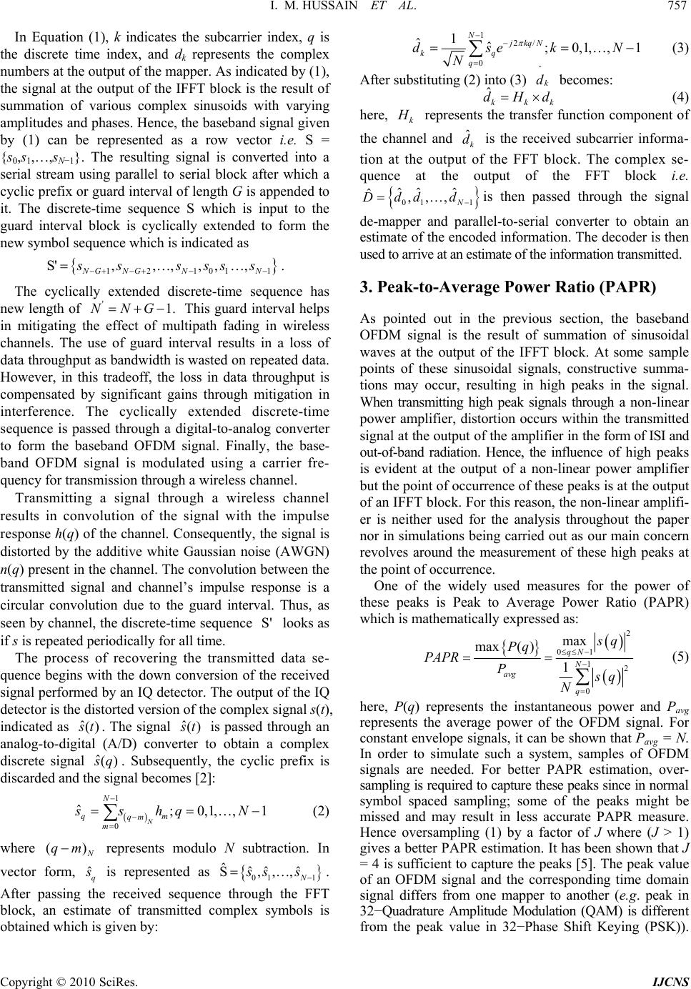

I. M. HUSSAIN ET AL. 757
In Equation (1), k indicates the subcarrier index, q is
the discrete time index, and d
k represents the complex
numbers at the output of the mapper. As indicated by (1),
the signal at the output of the IFFT block is the result of
summation of various complex sinusoids with varying
amplitudes and phases. Hence, the baseband signal given
by (1) can be represented as a row vector i.e. S =
{s0,s1,…,sN−1}. The resulting signal is converted into a
serial stream using parallel to serial block after which a
cyclic prefix or guard interval of length G is appended to
it. The discrete-time sequence S which is input to the
guard interval block is cyclically extended to form the
new symbol sequence which is indicated as


12101 1
S',,,, ,,
NG NGNN
ss ssss
 
.
The cyclically extended discrete-time sequence has
new length of '1.NNG This guard interval helps
in mitigating the effect of multipath fading in wireless
channels. The use of guard interval results in a loss of
data throughput as bandwidth is wasted on repeated data.
However, in this tradeoff, the loss in data throughput is
compensated by significant gains through mitigation in
interference. The cyclically extended discrete-time
sequence is passed through a digital-to-analog converter
to form the baseband OFDM signal. Finally, the base-
band OFDM signal is modulated using a carrier fre-
quency for transmission through a wireless channel.
Transmitting a signal through a wireless channel
results in convolution of the signal with the impulse
response h(q) of the channel. Consequently, the signal is
distorted by the additive white Gaussian noise (AWGN)
n(q) present in the channel. The convolution between the
transmitted signal and channel’s impulse response is a
circular convolution due to the guard interval. Thus, as
seen by channel, the discrete-time sequence S' looks as
if s is repeated periodically for all time.
The process of recovering the transmitted data se-
quence begins with the down conversion of the received
signal performed by an IQ detector. The output of the IQ
detector is the distorted version of the complex signal s(t),
indicated as ˆ()
s
t. The signal ˆ()
s
t is passed through an
analog-to-digital (A/D) converter to obtain a complex
discrete signal ˆ()
s
q. Subsequently, the cyclic prefix is
discarded and the signal becomes [2]:

1
0
;0,
ˆ1, ,1
N
N
qm qm
m
shqsN




 (2)
where ()
N
qm represents modulo N subtraction. In
vector form, ˆq
s
is represented as


01 1
ˆˆˆ ˆ
S,,,
N
ss s

 .
After passing the received sequence through the FFT
block, an estimate of transmitted complex symbols is
obtained which is given by:
12/
0
1;0,1, 1
ˆˆ,
NjkqN
kq
q
dsekN
N





 (3)
After substituting (2) into (3) k d

becomes:
ˆkkk
H
dd

 (4)
here, k
H
represents the transfer function component of
the channel and ˆk d is the received subcarrier informa-
tion at the output of the FFT block. The complex se-
quence at the output of the FFT block i.e.


01 1
ˆˆ ˆ,,, ˆN
dDdd


is then passed through the signal
de-mapper and parallel-to-serial converter to obtain an
estimate of the encoded information. The decoder is then
used to arrive at an estimate of the information transmitted.
3. Peak-to-Average Power Ratio (PAPR)
As pointed out in the previous section, the baseband
OFDM signal is the result of summation of sinusoidal
waves at the output of the IFFT block. At some sample
points of these sinusoidal signals, constructive summa-
tions may occur, resulting in high peaks in the signal.
When transmitting high peak signals through a non-linear
power amplifier, distortion occurs within the transmitted
signal at the output of the amplifier in the form of ISI and
out-of-band radiation. Hence, the influence of high peaks
is evident at the output of a non-linear power amplifier
but the point of occurrence of these peaks is at the output
of an IFFT block. For this reason, the non-linear amplifi-
er is neither used for the analysis throughout the paper
nor in simulations being carried out as our main concern
revolves around the measurement of these high peaks at
the point of occurrence.
One of the widely used measures for the power of
these peaks is Peak to Average Power Ratio (PAPR)
which is mathematically expressed as:
 

2
01
12
0
max
max( )
1
qN
N
avg
q
s
q
Pq
PAPR P
s
q
N
 




(5)
here, P(q) represents the instantaneous power and Pavg
represents the average power of the OFDM signal. For
constant envelope signals, it can be shown that Pavg = N.
In order to simulate such a system, samples of OFDM
signals are needed. For better PAPR estimation, over-
sampling is required to capture these peaks since in normal
symbol spaced sampling; some of the peaks might be
missed and may result in less accurate PAPR measure.
Hence oversampling (1) by a factor of J where (J > 1)
gives a better PAPR estimation. It has been shown that J
= 4 is sufficient to capture the peaks [5]. The peak value
of an OFDM signal and the corresponding time domain
signal differs from one mapper to another (e.g. peak in
32−Quadrature Amplitude Modulation (QAM) is different
from the peak value in 32−Phase Shift Keying (PSK)).

758 I. M. HUSSAIN ET AL.
For all phase shift keying, the maximum peak has the
value of N2 and hence a maximum PAPR of N. Figure 2
shows all possible OFDM signals for N = 4 and BPSK
mapper. It can be seen that the maximum normalized
absolute peak in such signals is 4 as indicated in the se-
quences 0000, 1001, 1010 and 1111.
Since the transmitted bits are generated randomly, the
transmitted OFDM signals are random in nature and
therefore the envelope of an OFDM signal, as given by
(1), can be considered a random variable. For large values
of N, according to the central limit theorem, the expected
amplitudes of OFDM signals follow a Gaussian distribution.
In addition, P(q) has a Chi square probability density
function with two degrees of freedom [5]. The PAPR
performance of a system is usually measured by the
Complementary Cumulative Distribution Function (CCD
F) curves, a standard way of depicting and describing
PAPR related statistics. The CCDF shows the probability
of an OFDM sequence exceeding a given PAPR (PAP0).
For PAPR, the lower bound on CCDF for a specific
PAPR value (i.e., PAP0) is given by [7]:


0
Pr
P
APR PAP  
This results in the following relationship:


0
11 N
PAP
e 

  (6)
4. Techniques for Minimizing PAPR
The objective is to minimize PAPR as much as possible
so as to obtain signals with smaller peaks. Various algo-
rithms and methods have been proposed for reducing
PAPR. One simple method for reducing PAPR is direct
clipping of high peaks and subsequent filtering of the
signal [7,8]. In addition, various modulation schemes are
used for efficient transmission of signals such as Conti-
nuous Phase Modulation (CPM) [9,10].
Recently, constellation and shaping methods have
Figure 2. Peak values in OFDM signals for N = 4 by using
BPSK mapper.
been used to reduce PAPR. In these methods, a mapping
between the original complex numbers and the finally
transmitted complex numbers takes place based on an
algorithm or a coding technique. One such method is the
trellis shaping method using a metric which is based on
the Viterbi algorithm [11]. One of the variants of this
method uses a metric-based symbol predistortion algo-
rithm resulting in some implementation complexity [12].
Another promising technique for reducing PAPR in-
volves scrambling the incoming OFDM sequence using
some rotation vectors resulting in multiple signals that
represent the same original information. Among these
signals, the signal with the lowest PAPR is transmitted.
Examples of such methods are Selected Mapping (SLM)
[13-15] and Partial Transmit Sequence (PTS) [16,17]. In
SLM, shown in Figure 3(a), from a single OFDM
sequence of length N, U sequences are generated that
represent the original information or OFDM sequence.
The sequence having lowest PAPR value is transmitted.
These sequences are generated by multiplying the original
OFDM sequence with U different factors. These factors
are given in vector form as ()() ()()
01 1
,,,
iiii
N
Bbbb




where i = 1 to U represents the indices of these factors.
After multiplying these factors by the original OFDM
sequence D, we get
 
00111 1
,,,
iii i
NN
Xdbdbdb




.
These factors are phase rotations selected appropriately
such that multiplying a complex number by these factors
(a)
(b)
Figure 3. The SLM method (a) at the transmitter and (b) at
the receiver.

I. M. HUSSAIN ET AL.
759
results in rotation of that complex number to another
complex number representing a different point in the
constellation. Hence, ()
() i
n
j i
n
be
 
 where () [0,2 )
i
n

 .
At the receiver end as shown in Figure 3(b), the orig-
inal OFDM sequence is recovered by multiplying the
received sequence by the reciprocal of the vector being
used at the transmitter end. Hence, in SLM, it is essential
to transmit the rotational vector B(i) as side information to
recover the original sequence.
On the other hand, in PTS method, as shown in Figure
4, the original OFDM sequence D is first partitioned into
H disjoint sub-sequences. The length of each sub-
sequence is still N but padded with zeros. Each sub-
sequence is fed into a separate IFFT block of length N
each. Hence, there are H number of IFFT blocks. The set
of complex numbers at the output of each IFFT block is
multiplied by a factor belonging to one of the rotation
factors as indicated in SLM technique. These factors are
optimized in such a manner that the PAPR of the com-
bined sub-sequences are reduced. After multiplying by
the factors, the complex numbers from all the IFFT
blocks are added together carrier-wise, resulting in a
final sequence. This final sequence has lower PAPR than
the original one.
Many other proposed algorithms tackle different
parameters for reducing the PAPR indirectly. One such
method is the Aperiodic Autocorrelation Coefficient
(AAC) of the transmitted OFDM signals in which PAPR
reduction is achieved using selective scrambling of the
transmitted sequence, generating a number of statistically
independent sequences [2]. A Selective Function (SF) is
computed for every sequence and the sequence with the
lowest SF, which also corresponds to the lowest PAPR,
is transmitted.
Another factor that plays an important role in reducing
Figure 4. PTS method.
PAPR is the Power Variance (PV) of an OFDM se-
quence. It is indicated in the literature that there exists a
strong relationship among AAC, PV and PAPR [2-4,20-
23,26]. In the next section, we study this relationship in
OFDM signals.
5. PV and Aperiodic Autocorrelation
Coefficients
For a complex envelope signal given by (1), the instan-
taneous power is given as:




*
PqqS q (7)
where ‘*’ denotes conjugate of a complex signal. By
combining (1) and (7) we get:

22
11 *
00
1
j
kqj pq
NN
NN
kp
kp
Pqdede
N
 


 (8)
Since the subcarriers in the OFDM signal are ortho-
gonal, they satisfy the following condition [2]:
 
1
*
0
0,
Φ,Φ,,
N
q
ij
iqjq Nij






 (9)
such that,
2
2/2( 1)/
2( 1)/2( 1)/
11 1
1
Φ
1
jNjN N
jN NjNN
ee
ee





















 

(10)
By simple manipulation of (8) and using the orthogonality
property of the subcarriers given by (9), the instantaneous
power can be expressed as:

22
11
*
0
11
1jiq jiq
NN
NN
ii
ii
PqR ReRe
N











 (11)
where Ri is called the ith Aperiodic Autocorrelation
Co-efficient of the complex OFDM sequence D and
given as [3]:
1
*
0
;0 1
Ni
ikki
k
RddiN




 
 (12)
Note that for i = 0, (12) becomes
12
0
N
kavg
ko
RdP



.
in case of a constant envelope mapper, Pavg = N. By com-
bining (11) and (12) then dividing by Pavg, we get the
normalized instantaneous power γ(q) given below:



avg
Pq
qP
 
1
1
1*
1
122
cos sin
22
cos sin
N
i
i
avg
N
i
i
iq iq
NR j
NPN N
iq iq
Rj
NN









 




 
 




 

 
 
 




hence, γ(q) is given by:

760 I. M. HUSSAIN ET AL.



11
*
11
122
2Re cos2Imsin
NN
ii
ii
avg
q
iq iq
NRR
NPN N






 

  
 


(13)
In compact form, (13) can be reduced into:



*
1
1
0
1
12
2cos tan
Re
Ni
i
i
avg i
Img R
iq
qRR
NPN R










 
 





(14)
Using Chebyshev polynomials, an upper bound on (14)
is given by [19]:

1
0
1
1
Γ2
N
i
i
avg
qRR
NP










 (15)
By taking the difference between the instantaneous
power and the average power, i.e. ΔP(q) = P(q) − Pavg,
we get the Power Variance of OFDM signal using the
following expression:

12
0
1N
q
PVP q
N








which can be further expanded using trigonometric
properties into the following expression:

11
2
11
12
1
14
22
cos cos1
Nm
im
iN
N
imavg
q
PVR R
NN
iqmq NP
NN











 


 
 



(16)
Hence, an upper limit on (16) becomes:
12
0
N
norm i
i
PV PVR



 (17)
here, PVnorm is the normalized power variance. It can be
observed from (11-15) that P(q), γ(q) and Γ are all func-
tions of AAC. Low values of |Ri| correspond to low in-
stantaneous power and hence low values of Γ. Based on
this assessment, some authors use (15) as a parameter for
measuring and comparing PAPR values of OFDM se-
quences. In contrast, other authors show that PAPR
analysis based on (14) and (15) gives misleading results
[19]. Through an example, they show that sequences
exist that have low PAPR values but high Γ values and
vice versa. They conclude that Γ cannot serve as para-
meters for PAPR comparison of sequences and hence Γ
is not a good measure for PAPR. In addition, many
authors concluded that PV is also a good measure of
PAPR [2-4,20-23]. However, in subsequent paragraphs,
we show that this is not always the case.
Figures 5 and 6 show normalized PAPR and PV values
respectively for different sets of 300 randomly generated
OFDM sequences when eight subcarriers are used. Ap-
parently, these figures suggest that PV is a good measure
Figure 5. Normalized PAPR for randomly generated
OFDM sequences with 8 subc ar riers.
Figure 6. Normalized PV for randomly generated OFDM
sequences with 8 subcarriers.
of PAPR as the pattern of both the figures for the same
set of symbols is almost the same. Hence, many authors
concluded that PV is a good measure for PAPR
[2-4,20-23]. However, we here demonstrate that this
observation is misleading because not all low PAPR
sequences have low PV and vice versa. To refute this
assertion, we investigate the relation between PV and
PAPR given as [4,5]:
11PAPR
QQ
PV PV






(18)
where Q(.)is the complementary error function and β
denotes Pr (P(q) ≤ P(q)max ) which is given by (6). Figure
7 shows a plot of (18) for selective values of PAPR for
256 subcarriers with β = 0.7434. Two aspects in this
Figure 7 are noteworthy. First, for a particular value of
PAPR, there are two values of PV. For instance, at PAPR
= 6.5 dB, the values of PV are 35 and 93.37. Second, PV
does not vary in proportion to PAPR. For instance, at
PAPR = 6dB, one of the values of PV is 79.89 whereas at
PAPR = 7dB, one of the values of PV is 44.31, i.e. an in-

I. M. HUSSAIN ET AL.
761
Figure 7. Relationship between PAPR and PV for β =
0.7434 with 256 subcarriers.
crease in PAPR does not always correspond to an in-
crease in PV. It shows that PV cannot always constitute a
basis for comparison of PAPR between two sequences.
Hence, PV cannot be considered a reliable measure for
PAPR. In addition, to emphasize our assessment of rela-
tionship between PV and PAPR, CCDF plots are used
for PAPR measure based on PV using SLM and PTS
techniques.
In the first simulation experiment, CCDF curves are
plotted for 50,000 randomly generated OFDM sequences
using SLM technique where U = 4, 16 and 64 as shown
in Figure 8. In this approach, U different sequences are
generated from a single OFDM sequence D using ran-
domly generated phase rotation factors. The sequences
having the lowest PV and the lowest PAPR are selected
for transmission. In short, the selection decision for
transmitting a sequence is based on both the lowest PV
and the lowest PAPR. This simulation gives two sets of
CCDF curves, as shown in Figure 8. It is clear that the
reduction in PAPR based on PV is not the same as the
one based on PAPR. For instance at CCDF = 0.001,
when U = 64, the PAPR reduction using a PV-based de-
cision is approximately 2dB while the PAPR reduction
based on PAPR itself is around 3.8dB. A difference of
almost 2dB is evident between the two transmission
decisions. This difference in PAPR reduction is suffi-
cient to show that PV is not a good and reliable measure
for the purposes of PAPR reduction.
For the second simulation experiment, CCDF curves
are plotted for 50,000 randomly generated OFDM se-
quences using PTS technique using 256 subcarriers and
H = 16, shown in Figure 9. As it is the case in SLM, two
curves are generated for both PV- and PAPR-based
transmission decisions. A PAPR reduction of 2dB is
achieved in case of PV-based decision whereas a reduc-
tion of 3.5dB is achieved in case of PAPR-based decision.
Once again, the difference in PAPR performance be-
Figure 8. CCDF curves for SLM based on PAPR and PV
for various values of U.
Figure 9. CCDF curves for PTS technique based on PAPR
and PV for H = 16.
tween PV-based and PAPR-based transmission decisions
is significant and obvious. All these results suggest that
low values of PV do not always correspond to low PAPR
values and vice versa. Consequently, PV is not a reliable
measure of PAPR and it cannot be used as a parameter
for OFDM sequence selection in both SLM and PTS
techniques. Since OFDM sequences follow a random
process, it is difficult to tell the range of PAPR values or
sequences that correspond to high PV values and vice
versa.
It can also be noted that for a particular number of
subcarriers N, the values of β vary with PAPR values.
Although theoretically PAPR, PV and β can take any
value, as indicated by (18), the actual values of these
three parameters are finite and specific for a given num-
ber of subcarriers. For instance, through simulation we
generate all possible OFDM symbols for 16 subcarriers
using BPSK mapper and plot their corresponding PAPR
values against PV values as shown in Figure 10. The
total number of possible OFDM symbols is 65,536. The
maximum and minimum PAPR values are 16 and 1.7071
respectively and the corresponding PV values for these
PAPR values are 1240 and 24 respectively. Note that the
plot is discontinuous through PAPR axis because the

762 I. M. HUSSAIN ET AL.
Figure 10. PV versus PAPR values for OFDM sequences
with 16 subcarrier s and BP SK mapper .
OFDM symbols have finite and specific values of PAPR,
as mentioned earlier.
It is interesting to note that our assessment regarding
the relation between PV and PAPR is more pronounced
for low values of PAPR than high values of PAPR (i.e.
more concentration of points in the lower region of
PAPR). It can be seen that for a single PAPR value in the
lower range (approximately from 2dB to 5dB), there are
more than one corresponding PV value. Similarly, for a
single value of PV (approximately from 24 to 300), there
are more than one corresponding PAPR value. Again,
this plot is only possible for small number of subcarriers.
For high number of subcarriers, it is difficult to find the
distribution of PAPR and PV values for all possible OFDM
sequences.
6. Computational Complexity of PV
SLM algorithm based on PAPR comparison has moderate
complexity. The main complexity is based on the com-
putation of IFFT operation. This complexity increases as
U increases. Hence, IFFT has to be computed for every
sequence (i.e. U times) before transmitting the final
selected sequence. Similarly, when evaluating PV, Equa-
tion (17) needs to be evaluated for every sequence (i.e. U
times) before transmitting the final selected sequence. So,
it would be interesting to compare the complexity asso-
ciated with computing PAPR with the complexity in
evaluating PV.
The complexity expressions in terms of complex addi-
tions and multiplications for evaluating IFFT, and there-
fore PAPR, are shown in Table 1 [28]. Similarly it could
easily be shown that the complexity for evaluating Equa-
tion (17) in terms of both complex additions and multip-
lications is given as:


12
2
11
2
NN
Complex Additions
N
ComplexMultiplicationsN
 






 




(19)
Table 1. Computational complexity of various parameters.
ExpressionComplex Additions Complex Multiplica-
tions
IFFT JN(log2JN) JN(log2JN) ⁄ 2
IFFT and
PAPR JN(log2JN) (JN(log2JN) ⁄ 2) + JN
PV (N (N − 1) – 2 ) ⁄ 2 (N − 1) ( (N ⁄ 2) + 1)
PPV (B (2N–B−1)−2) ⁄ 2 (B (2N–B−1) ⁄ 2) + B
Table 2. Computational complexity of various parameters
for different subcarriers.
N
Complex Additions
PAPR
(J = 1)
PAPR (J
= 4) PV PPV (B) PPV (B = 1)
4 8 64 5 4 (2) 2
8 24 160 27 21 (4) 6
1664 384 119 91 (8) 14
32160 896 495 219 (8) 30
64384 2048 2015 475 (8) 62
128896 4608 8127 1911 (16) 126
2562048 10240 32639 3959 (16) 254
N
Complex Multiplications
PAPR (J
= 1)
PAPR (J
= 4) PV PPV (B) PPV (B = 1)
4 4 32 9 7 (2) 4
8 12 80 35 26 (4) 8
1632 192 135 100 (8) 16
3280 448 527 228 (8) 32
64192 1024 2079 448 (8) 64
128448 2304 8255 1928 (16) 128
2561024 5120 32895 3976 (16) 256
The computational complexity for both PAPR and PV
for different values of N is presented in Table. 2. Note
that, for comparison purposes, PAPR complexity is also
evaluated when oversampling OFDM signals by a factor
of 4. It is clear that the computational complexity of PV
is lower than that of PAPR only for very small values of
N (i.e. N = 2 and 4). For large values of N, the computa-
tional complexity of PV is far greater than that of PAPR
complexity even when J = 4. Hence, PV-based selection
becomes impractical for large values of N. This is another
disadvantage of using PV as a selection criterion in SLM
or PTS techniques, pronouncing the need for an efficient
measure of PAPR. In the next section, we propose one
such measure of PAPR
7. AAC-SLM Algorithm and Partial Power
Variance (PPV)
In this section, we introduce a new parameter called Par-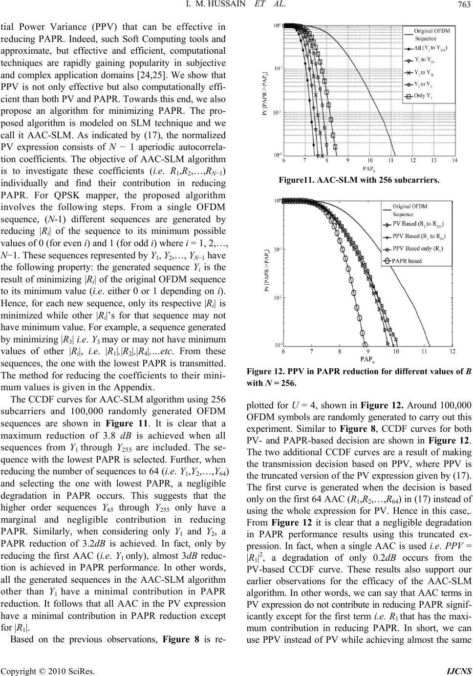

I. M. HUSSAIN ET AL.
763
tial Power Variance (PPV) that can be effective in
reducing PAPR. Indeed, such Soft Computing tools and
approximate, but effective and efficient, computational
techniques are rapidly gaining popularity in subjective
and complex application domains [24,25]. We show that
PPV is not only effective but also computationally effi-
cient than both PV and PAPR. Towards this end, we also
propose an algorithm for minimizing PAPR. The pro-
posed algorithm is modeled on SLM technique and we
call it AAC-SLM. As indicated by (17), the normalized
PV expression consists of N − 1 aperiodic autocorrela-
tion coefficients. The objective of AAC-SLM algorithm
is to investigate these coefficients (i.e. R1,R2,…,RN−1)
individually and find their contribution in reducing
PAPR. For QPSK mapper, the proposed algorithm
involves the following steps. From a single OFDM
sequence, (N-1) different sequences are generated by
reducing |Ri| of the sequence to its minimum possible
values of 0 (for even i) and 1 (for odd i) where i = 1, 2,…,
N−1. These sequences represented by Y1, Y2,…, YN−1 have
the following property: the generated sequence Yi is the
result of minimizing |Ri| of the original OFDM sequence
to its minimum value (i.e. either 0 or 1 depending on i).
Hence, for each new sequence, only its respective |Ri| is
minimized while other |Ri|’s for that sequence may not
have minimum value. For example, a sequence generated
by minimizing |R3| i.e. Y3 may or may not have minimum
values of other |Ri|, i.e. |R1|,|R2|,|R4|,…etc. From these
sequences, the one with the lowest PAPR is transmitted.
The method for reducing the coefficients to their mini-
mum values is given in the Appendix.
The CCDF curves for AAC-SLM algorithm using 256
subcarriers and 100,000 randomly generated OFDM
sequences are shown in Figure 11. It is clear that a
maximum reduction of 3.8 dB is achieved when all
sequences from Y1 through Y
255 are included. The se-
quence with the lowest PAPR is selected. Further, when
reducing the number of sequences to 64 (i.e. Y1,Y2,…,Y64)
and selecting the one with lowest PAPR, a negligible
degradation in PAPR occurs. This suggests that the
higher order sequences Y65 through Y
255 only have a
marginal and negligible contribution in reducing
PAPR. Similarly, when considering only Y1 and Y
2, a
PAPR reduction of 3.2dB is achieved. In fact, only by
reducing the first AAC (i.e. Y1 only), almost 3dB reduc-
tion is achieved in PAPR performance. In other words,
all the generated sequences in the AAC-SLM algorithm
other than Y1 have a minimal contribution in PAPR
reduction. It follows that all AAC in the PV expression
have a minimal contribution in PAPR reduction except
for |R1|.
Based on the previous observations, Figure 8 is re-
Figure11. AAC-SLM with 256 subcarriers.
Figure 12. PPV in PAPR reduction for different values of B
with N = 256.
plotted for U = 4, shown in Figure 12. Around 100,000
OFDM symbols are randomly generated to carry out this
experiment. Similar to Figure 8, CCDF curves for both
PV- and PAPR-based decision are shown in Figure 12.
The two additional CCDF curves are a result of making
the transmission decision based on PPV, where PPV is
the truncated version of the PV expression given by (17).
The first curve is generated when the decision is based
only on the first 64 AAC (R1,R2,…,R64) in (17) instead of
using the whole expression for PV. Hence in this case,.
From Figure 12 it is clear that a negligible degradation
in PAPR performance results using this truncated ex-
pression. In fact, when a single AAC is used i.e. PPV =
|R1|2, a degradation of only 0.2dB occurs from the
PV-based CCDF curve. These results also support our
earlier observations for the efficacy of the AAC-SLM
algorithm. In other words, we can say that AAC terms in
PV expression do not contribute in reducing PAPR signif-
icantly except for the first term i.e. R1 that has the maxi-
mum contribution in reducing PAPR. In short, we can
use PPV instead of PV while achieving almost the same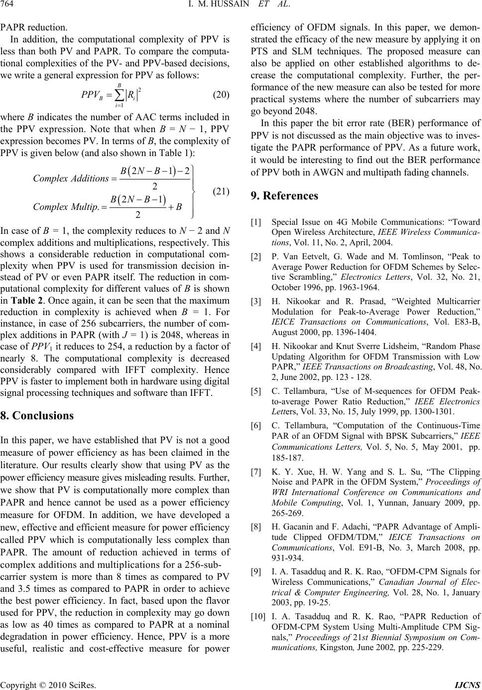

764 I. M. HUSSAIN ET AL.
PAPR reduction.
In addition, the computational complexity of PPV is
less than both PV and PAPR. To compare the computa-
tional complexities of the PV- and PPV-based decisions,
we write a general expression for PPV as follows:
2
1
B
B
i
i
PPV R

 (20)
where B indicates the number of AAC terms included in
the PPV expression. Note that when B = N − 1, PPV
expression becomes PV. In terms of B, the complexity of
PPV is given below (and also shown in Table 1):



212
2
21
.2
BNB
Complex Additions
BNB
ComplexMultipB
 









(21)
In case of B = 1, the complexity reduces to N − 2 and N
complex additions and multiplications, respectively. This
shows a considerable reduction in computational com-
plexity when PPV is used for transmission decision in-
stead of PV or even PAPR itself. The reduction in com-
putational complexity for different values of B is shown
in Table 2. Once again, it can be seen that the maximum
reduction in complexity is achieved when B = 1. For
instance, in case of 256 subcarriers, the number of com-
plex additions in PAPR (with J = 1) is 2048, whereas in
case of PPV1 it reduces to 254, a reduction by a factor of
nearly 8. The computational complexity is decreased
considerably compared with IFFT complexity. Hence
PPV is faster to implement both in hardware using digital
signal processing techniques and software than IFFT.
8. Conclusions
In this paper, we have established that PV is not a good
measure of power efficiency as has been claimed in the
literature. Our results clearly show that using PV as the
power efficiency measure gives misleading results. Further,
we show that PV is computationally more complex than
PAPR and hence cannot be used as a power efficiency
measure for OFDM. In addition, we have developed a
new, effective and efficient measure for power efficiency
called PPV which is computationally less complex than
PAPR. The amount of reduction achieved in terms of
complex additions and multiplications for a 256-sub-
carrier system is more than 8 times as compared to PV
and 3.5 times as compared to PAPR in order to achieve
the best power efficiency. In fact, based upon the flavor
used for PPV, the reduction in complexity may go down
as low as 40 times as compared to PAPR at a nominal
degradation in power efficiency. Hence, PPV is a more
useful, realistic and cost-effective measure for power
efficiency of OFDM signals. In this paper, we demon-
strated the efficacy of the new measure by applying it on
PTS and SLM techniques. The proposed measure can
also be applied on other established algorithms to de-
crease the computational complexity. Further, the per-
formance of the new measure can also be tested for more
practical systems where the number of subcarriers may
go beyond 2048.
In this paper the bit error rate (BER) performance of
PPV is not discussed as the main objective was to inves-
tigate the PAPR performance of PPV. As a future work,
it would be interesting to find out the BER performance
of PPV both in AWGN and multipath fading channels.
9. References
[1] Special Issue on 4G Mobile Communications: “Toward
Open Wireless Architecture, IEEE Wireless Communica-
tions, Vol. 11, No. 2, April, 2004.
[2] P. Van Eetvelt, G. Wade and M. Tomlinson, “Peak to
Average Power Reduction for OFDM Schemes by Selec-
tive Scrambling,” Electronics Letters, Vol. 32, No. 21,
October 1996, pp. 1963-1964.
[3] H. Nikookar and R. Prasad, “Weighted Multicarrier
Modulation for Peak-to-Average Power Reduction,”
IEICE Transactions on Communications, Vol. E83-B,
August 2000, pp. 1396-1404.
[4] H. Nikookar and Knut Sverre Lidsheim, “Random Phase
Updating Algorithm for OFDM Transmission with Low
PAPR,” IEEE Transactions on Broadcasting, Vol. 48, No.
2, June 2002, pp. 123 - 128.
[5] C. Tellambura, “Use of M-sequences for OFDM Peak-
to-average Power Ratio Reduction,” IEEE Electronics
Letters, Vol. 33, No. 15, July 1999, pp. 1300-1301.
[6] C. Tellambura, “Computation of the Continuous-Time
PAR of an OFDM Signal with BPSK Subcarriers,” IEEE
Communications Letters, Vol. 5, No. 5, May 2001, pp.
185-187.
[7] K. Y. Xue, H. W. Yang and S. L. Su, “The Clipping
Noise and PAPR in the OFDM System,” Proceedings of
WRI International Conference on Communications and
Mobile Computing, Vol. 1, Yunnan, January 2009, pp.
265-269.
[8] H. Gacanin and F. Adachi, “PAPR Advantage of Ampli-
tude Clipped OFDM/TDM,” IEICE Transactions on
Communications, Vol. E91-B, No. 3, March 2008, pp.
931-934.
[9] I. A. Tasadduq and R. K. Rao, “OFDM-CPM Signals for
Wireless Communications,” Canadian Journal of Elec-
trical & Computer Engineering, Vol. 28, No. 1, January
2003, pp. 19-25.
[10] I. A. Tasadduq and R. K. Rao, “PAPR Reduction of
OFDM-CPM System Using Multi-Amplitude CPM Sig-
nals,” Proceedings of 21st Biennial Symposium on Com-
munications, Kingston, June 2002, pp. 225-229.

I. M. HUSSAIN ET AL.
765
[11] H. Ochiai, “A Novel Trellis-shaping Design with Both
Peak and Average Power Reduction for OFDM Sys-
tems,” IEEE Transactions on Communications, Vol. 52,
No. 11, November 2004, pp. 1916-1926.
[12] S. Sezginer and H. Sari, “Metric-Based Symbol Predis-
tortion Techniques for Peak Power Reduction in OFDM
Systems,” IEEE Transactions on Wireless Communica-
tions, Vol. 6, No. 7, July 2007, pp. 2622-2629.
[13] S. Yang and Y. Shin, “An Adaptive SLM Scheme Based
on Peak Observation for PAPR Reduction of OFDM
Signals,” IEICE Transactions on Fundamentals of Elec-
tronics, Communications and Computer Sciences, Vol.
E91, No. 1, January 2008, pp. 422-425.
[14] A. D. S. Jayalath and C. Tellambura “SLM and PTS
Peak-Power Reduction of OFDM Signals without Side
Information,” IEEE Transactions on Wireless Communica-
tions, Vol. 4, No. 5, September 2005. pp. 2006-2013.
[15] C. L. Wang and S. J. Ku, “Novel Conversion Matrices for
Simplifying the IFFT Computation of an SLM-Based
PAPR Reduction Scheme for OFDM Systems,” IEEE
Transactions on Communications, Vol. 57, No. 7, July
2009, pp. 1903-1907.
[16] L. Yanga, R. S. Chena, K. K. Soob and Y. M. Siub, “An
Efficient Sphere Decoding Approach for PTS Assisted
PAPR Reduction of OFDM Signals,” International
Journal of Electronics and Communications, Vol. 61, No.
10, November 2007, pp. 684-688.
[17] Y. Zhang, Q. Ni and H.-H. Chen, “A New Partial Trans-
mit Sequence Scheme Using Genetic Algorithm for
Peak-to-Average Power Ratio Reduction in a Mul-
ti-Carrier Code Division Multiple Access Wireless Sys-
tem,” International Journal of Autonomous and Adaptive
Communications Systems, Vol. 2, No. 1, March 2009, pp.
40-57.
[18] C. Tellambura, “Upper Bound on Peak Factor of
N-multiple Carriers,” Electronic Letters, Vol. 33, Sep-
tember 1997, pp. 1608-1609.
[19] N. Y. Ermolova and P. Vainikainen, “On the Relationship
between Peak Factor of a Multicarrier Signal and Aperiodic
Autocorrelation of the Generating Sequence,” IEEE Com-
munications Letters, Vol. 7, No. 3, March 2003, pp.
107-108.
[20] A. Ghassemi and T. A. Gulliver, “Low Autocorrelation
Fractional PTS Subblocking for PAPR Reduction in
OFDM Systems,” Proceedings of 6th Annual Conference
on Communication Networks and Services Research,
Nova Scotia, May 2008, pp. 41-45.
[21] C. Y. Hsu and H. Do, “The New Peak-to-Average Power
Reduction Algorithm in the OFDM System,” Wireless
Personal Communications, Vol. 41, No. 4, June 2007, pp.
517-525.
[22] E. Sun, K. Yi, B. Tian and X. Wang, “A Method for
PAPR Reduction in MSE-OFDM Systems,” Proceedings
of International Conference on Advanced Information
Networking and Applications 2006, Vienna, Vol. 2, April
2006, pp. 18-20.
[23] D. Wu, S. Predrag and S. Ivan, “Ternary Complementary
Sets for Multiple Channel DS-UWB with Reduced Peak-
to-Average Power Ratio,” Proceedings of IEEE GLOB
ECO, Texas, November 2004, pp. 3230-3234.
[24] A. R. Ahmad, O. Basir and K. Hassanein, “An Intelligent
Expert Systems Approach to Layout Decision Analysis
and Design Under Uncertainty,” Springer-Verlag, 2008,
pp. 312-365.
[25] A. R. Ahmad, “An Intelligent Expert System for Decision
Analysis & Support,” Ph.D. Thesis, University of Water-
loo, Waterloo.
[26] I. M. Hussain and I. A Tasadduq, “PAPR Analysis in
OFDM Signals Based on Power Variance,” Proceedings
of Wireless Communications, Networking and Mobile
Computing, Dalian, October 2008, pp. 1-4.
[27] M. Negnevitsky, “Artificial Intelligence: A Guide to In-
telligent Systems,” Pearson, Sydney, 2008.
[28] A. V. Oppenheim and R. W. Schafer, Discrete-Time Signal
Processing, Englewood Cliffs: Prentice Hall, 1989.

766 I. M. HUSSAIN ET AL.
Appendix
As indicated in (17), the normalized PV expression con-
tains N – 1 AAC terms. AAC term can be represented by
(12). In case of constant envelope mapper (e.g. QPSK
which is used throughout our simulations), (12) can be
modified into:
1
0
;0 1
Ni
k
i
kki
d
RiN
d




031 12
123 1
Ni
i
iii iN
ddd
dd
Rddd dd

 
 
 
 
 
 (22)
Hence each expression of Ri contains N − i terms of
kind (dk / dk+i) . Using (22) and (17) it can easily be
shown that the total number of such terms in the power
variance expression is 1
1
N
iNi


. Similarly, the total
number of pairs of adjacent terms in R
i as indicated by
parenthesis in (22) is /2Ni. Now one way to reduce
AAC to their minimum values (i.e. 0 or 1 depending on i)
is to make the summation of each and every pair of terms
in (22) equal to zero. Let 1
1
pp
pipi
dd
dd







be any pair in
(22) where p = 0,2,4,…,N – 2 – i (for even i) and p =
0,2,4,…,N – 3 – i (for odd i). In case of i = 1,2,3,…,N
– 1, to minimize the values of all such pairs to zero, we
have to multiply every second complex number (i.e.
subcarrier) starting from dp+i by a factor gi,v. This factor
is obtained as shown below:
For the first /2i number of pairs:
1
,1
0
pp
iv pipi
dd
gd d








1
,
1
;
p
pi
iv
p
pi
dd
gdd


 (23)
For rest of the pairs when i is even:
1
,
1
;
p
p
i
iv
p
pi
dd
gdd


 (24)
For rest of the pairs when i is odd
1
,
1
;
ppi
iv
ppi
dd
d
gd


 (25)
where
1
,/21 ,/2
,
pp
p
iv ipivi
dgd gdd


  and 1
2
p
v.
For example, in case of N = 16 subcarriers and i = 4,
the fourth AAC becomes:
03567 12 4
4
4 56 7891011
ddddd
dd d
Rdd dddd dd
 

 
 
89 10 11
12 131415
dd dd
dd dd




This expression has 6 pairs i.e.164 / 2 and as many
factors and each factor is used to minimize the corres-
ponding pair to zero. Since i is even, then p = 0,2,4,…,10.
For instance, the third pair in R4 is 5
4
89
d d
dd




where v =
3 and p = 4. In order to find the six factors used to mi-
nimize each pair, (23) is used for the first 2 pairs i.e.
05
4,1
14
dd
gdd  and 27
4,2
36
dd
gdd  . Rest of the factors are
calculated using (24) as i is even. Hence,
49
4,3
58
d
gd
dd

,
611
4,4
710
d
gd
d
d
 , 813
4,5
911
d
gd
d
d
 and
10 15
4,6
914
d
gd
d
d
 ,where 444,1 dd
g
 , 664,2 dd
g
 ,
884,3
dd
g
 and 10 104,4 dd
g
 . Further, each alter-
nate complex number starting from d4 (i.e. d4, d6, d8, d12,
d14, d16) will be multiplied by g4,1, g4,2, g4,3, g4,4, g4,5 and
g4,6 respectively. In this manner |R4| will be minimized to
zero. It is clear that p
d or 1p d means that before mi-
nimizing the corresponding pair to zero, updation of p d
into p d has to take place first. In the above example,
for the third pair, updation of d4 (i.e.444,1 dd
g
 ) has to
take place first after which minimization of that pair
takes place. Thus, the third pair has the form 45
89
dd
dd





rather than 5
4
89
d
d
dd




. Now in case of i = 1 i.e. R1
which is an exception case, factor expression is given by
(23) for the first pair and for the rest of the pairs, it is
given by (24) where ,1
p
p
iv
dgd  . Further, each com-
plex number starting from d1 is going to be multiplied by
the corresponding factor. In this manner, we can minim-
ize the coefficients of any sequence to their respective
minimum values using the procedure above.