Circuits and Systems, 2013, 4, 49-57
http://dx.doi.org/10.4236/cs.2013.41009 Published Online January 2013 (http://www.scirp.org/journal/cs)
Thermal Defect Analysis on Transformer Using a RLC
Network and Thermography
Geoffrey O. Asiegbu¹, Ahmed M. A. Haidar², Kamarul Hawari1
1Faculty of Electrical and Electronics Engineering, University Malaysia Pahang, Kuantan, Malaysia
2School of Electrical, Computer and Telecommunications Engineering, University of Wollongong, Wollongong, Australia
Received August 2, 2012; revised September 2, 2012; accepted September 10, 2012
ABSTRACT
Electrical transformers are vital components found virtually in most power-operated equipments. These transformers
spontaneously radiate heat in both operation and steady-state mode. Should this thermal radiation inherent in trans-
formers rises above allowable threshold a reduction in efficiency of operation occurs. In addition, this could cause other
components in the system to malfunction. The aim of this work is to detect the remote causes of this undesirable ther-
mal rise in transformers such as oil distribution transformers and ways to control this prevailing thermal problem. Oil
transformers consist of these components: windings usually made of copper or aluminum conductor, the core normally
made of silicon steel, the heat radiators, and the dielectric materials such as transformer oil, cellulose insulators and
other peripherals. The Resistor-Inductor-Capacitor Thermal Network (RLCTN) model at architectural level identifies
with these components to have ensemble operational mode as oil transformer. The Inductor represents the windings, the
Resistor representing the core and the Capacitor represents the dielectrics. Thermography of transformer under various
loading conditions was analyzed base on Infrared thermal gradient. Mathematical, experimental, and simulation results
gotten through RLCTN with respect to time and thermal image analysis proved that the capacitance of the dielectric is
inversely proportional to the thermal rise.
Keywords: Thermal Radiation; RLC Thermal Network; Thermography; Defect Analysis
1. Introduction
Sustainability is the intermediary that runs between
manufacturers of electrical equipments and her end-users.
For sustainability to achieve its desired goal, electrical
power facilities should be able to satisfy the demands of
the users. These does not mean that faults cannot occur in
equipments at any given time, however, certain electrical
faults can be avoided while causes of the rest can be mi-
nimized if attention to thermal effect is considered with
utmost importance. In order to throttle thermal variations
in transformers within a safe-steady-state, such current
dependent equipments also known as thermal producers
should be monitored and assisted to function efficiently
within their life span. The aim of using the Resis-
tor-Inductor-Capacitor Thermal Network (RLCTN) is to
track equipments exceeding thermal rise as early as pos-
sible by examining effects of thermal capacitance and
thermal resistance on oil transformers. Secondly, to de-
velop a mathematical model that helps in the study of
thermal characteristics of oil distribution transformer
components. Nearly every component gets hot before it
fails [1]. Therefore, abnormal thermal rise of even minor
piece of component could result to sudden failure and
great setback on production. So, causes of abnormal
thermal rise have to be addressed without hesitation.
Hence, RLCTN model is one of the appropriate measures
taken to ensure equipment durability.
Until date, many researchers have been battling with
heat management in electrical equipments, which are a
vital phenomenon affecting equipments performance,
sustainability and overall system efficiency. Generally,
increasing current 2
I
R that generates undesirable ther-
mal consequence in electrical equipments mainly occur
due to high current, and in some situations in the form of
free convection during thermal variations in the internal
and external surfaces of the current conducting parts un-
der different electrical loads and environment conditions
[2]. In many manufacturing operations, electrical power
systems have been the fundamental pillars whose contri-
butions cannot be overemphasized; adherence to IEEE
thermal evaluation regulations [3] will create an enabling
environment for electrical facilities to function maxi-
mally.
Obviously, most system faults were discovered when
thermal variation significantly deviates from its normal
thermal value(s). This can be figured out using delta T
C
opyright © 2013 SciRes. CS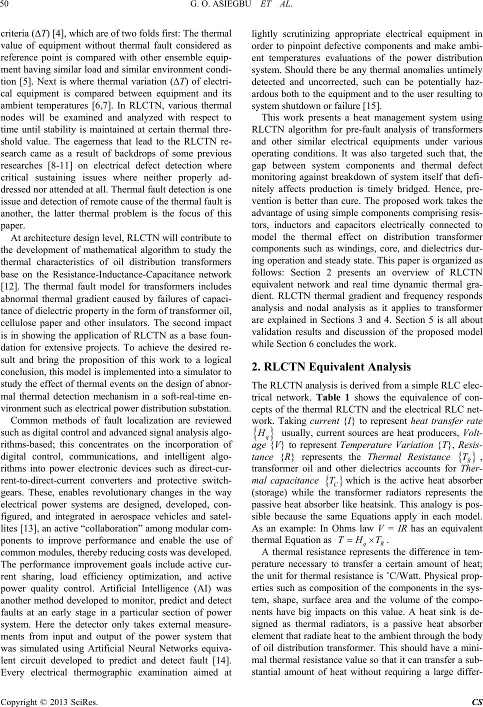

G. O. ASIEGBU ET AL.
50
criteria (∆T) [4], which are of two folds first: The thermal
value of equipment without thermal fault considered as
reference point is compared with other ensemble equip-
ment having similar load and similar environment condi-
tion [5]. Next is where thermal variation (∆T) of electri-
cal equipment is compared between equipment and its
ambient temperatures [6,7]. In RLCTN, various thermal
nodes will be examined and analyzed with respect to
time until stability is maintained at certain thermal thre-
shold value. The eagerness that lead to the RLCTN re-
search came as a result of backdrops of some previous
researches [8-11] on electrical defect detection where
critical sustaining issues where neither properly ad-
dressed nor attended at all. Thermal fault detection is one
issue and detection of remote cause of the thermal fault is
another, the latter thermal problem is the focus of this
paper.
At architecture design level, RLCTN will contribute to
the development of mathematical algorithm to study the
thermal characteristics of oil distribution transformers
base on the Resistance-Inductance-Capacitance network
[12]. The thermal fault model for transformers includes
abnormal thermal gradient caused by failures of capaci-
tance of dielectric property in the form of transformer oil,
cellulose paper and other insulators. The second impact
is in showing the application of RLCTN as a base foun-
dation for extensive projects. To achieve the desired re-
sult and bring the proposition of this work to a logical
conclusion, this model is implemented into a simulator to
study the effect of thermal events on the design of abnor-
mal thermal detection mechanism in a soft-real-time en-
vironment such as electrical power distribution substation.
Common methods of fault localization are reviewed
such as digital control and advanced signal analysis algo-
rithms-based; this concentrates on the incorporation of
digital control, communications, and intelligent algo-
rithms into power electronic devices such as direct-cur-
rent-to-direct-current converters and protective switch-
gears. These, enables revolutionary changes in the way
electrical power systems are designed, developed, con-
figured, and integrated in aerospace vehicles and satel-
lites [13], an active “collaboration” among modular com-
ponents to improve performance and enable the use of
common modules, thereby reducing costs was developed.
The performance improvement goals include active cur-
rent sharing, load efficiency optimization, and active
power quality control. Artificial Intelligence (AI) was
another method developed to monitor, predict and detect
faults at an early stage in a particular section of power
system. Here the detector only takes external measure-
ments from input and output of the power system that
was simulated using Artificial Neural Networks equiva-
lent circuit developed to predict and detect fault [14].
Every electrical thermographic examination aimed at
lightly scrutinizing appropriate electrical equipment in
order to pinpoint defective components and make ambi-
ent temperatures evaluations of the power distribution
system. Should there be any thermal anomalies untimely
detected and uncorrected, such can be potentially haz-
ardous both to the equipment and to the user resulting to
system shutdown or failure [15].
This work presents a heat management system using
RLCTN algorithm for pre-fault analysis of transformers
and other similar electrical equipments under various
operating conditions. It was also targeted such that, the
gap between system components and thermal defect
monitoring against breakdown of system itself that defi-
nitely affects production is timely bridged. Hence, pre-
vention is better than cure. The proposed work takes the
advantage of using simple components comprising resis-
tors, inductors and capacitors electrically connected to
model the thermal effect on distribution transformer
components such as windings, core, and dielectrics dur-
ing operation and steady state. This paper is organized as
follows: Section 2 presents an overview of RLCTN
equivalent network and real time dynamic thermal gra-
dient. RLCTN thermal gradient and frequency responds
analysis and nodal analysis as it applies to transformer
are explained in Sections 3 and 4. Section 5 is all about
validation results and discussion of the proposed model
while Section 6 concludes the work.
2. RLCTN Equivalent Analysis
The RLCTN analysis is derived from a simple RLC elec-
trical network. Table 1 shows the equivalence of con-
cepts of the thermal RLCTN and the electrical RLC net-
work. Taking current {I} to represent heat transfer rate


q
H
usually, current sources are heat producers, Volt-
age {V} to represent Temperature Variation {T}, Resis-
tance {R} represents the Thermal Resistance


R
T,
transformer oil and other dielectrics accounts for Ther-
mal capacitance


T
THT
Cwhich is the active heat absorber
(storage) while the transformer radiators represents the
passive heat absorber like heatsink. This analogy is pos-
sible because the same Equations apply in each model.
As an example: In Ohms law V = IR has an equivalent
thermal Equation as qR .


A thermal resistance represents the difference in tem-
perature necessary to transfer a certain amount of heat;
the unit for thermal resistance is ˚C/Watt. Physical prop-
erties such as composition of the components in the sys-
tem, shape, surface area and the volume of the compo-
nents have big impacts on this value. A heat sink is de-
signed as thermal radiators, is a passive heat absorber
element that radiate heat to the ambient through the body
of oil distribution transformer. This should have a mini-
mal thermal resistance value so that it can transfer a sub-
stantial amount of heat without requiring a large differ-

G. O. ASIEGBU ET AL. 51
ence in temperature. Because of this, the air gap or space
between the radiator fins, type of material and size are
importantly considered. Capacitor in this thermal analy-
sis network plays the role of active heat absorber meas-
ured in Joule per degree centigrade, i.e., J/˚C. The ca-
pacitance is a measure of the amount of thermal energy
that is stored or removed to increase or decrease the
thermal flow within the oil distribution transformer that
depends largely on the heat absorbent or storage capacity,
type of materials such as oil viscosity, quality of cellu-
lous paper and conductor insulators, then volume and
size of the oil container. The above analogy describes the
thermal properties as a system of linear differential equa-
tions that will be detailed in the subsequent sections of
this paper; a popular technique widely adopted in most
circuitries, mainly in electrical and electronic engineering
designs. This very simple thermal RLCTN can analyze
and predict the dynamic behavior of real-time oil distri-
bution transformer as shown in Figure 1 [16].
3. Thermal Gradient Analysis
RLCTN approach is used for instantaneous thermal
analysis of electrical distribution substation transformer.
The idea of using RLCTN for analyzing thermal effect is
Table 1. Comparison of thermal network to electrical net-
work.
Thermal Network Electrical Network
Temperature (˚C) TVoltage V (Volt)
Heat Transfer Rate q
H
(Watt) Current I (Ampere)
Thermal Resistance
R
T (˚C/Watt) Resistance R (Ohms)
Thermal Inductance
L
T
C
T
S
T
S
Inductance L (Henry)
Thermal Capacitance (J/˚C) Capacitance C (Coulomb/Volt)
Temperature Source Voltage Source
Heat Source
H
Current Source
Figure 1. Dynamic thermal gradient of oil transformer.
not new but an analytical algorithm that describes every
individual component with respect to the thermal char-
acteristics of most current dependent or current sourcing
equipment such as oil distribution transformer. In every
electrical distribution substation, there exists lots of heat
dissipating components comprising of instantaneous
elements arranged for efficient generation of electric
power. RLCTN as the name implies is reasonably less
cumbersome and less complexity due to small number of
components are used, which is quite imperative for on-
line computation and for prediction of future thermal
variations at all levels. This thermal analysis incorporates
heat producers for example, transformer windings repre-
sented as inductors; core represented as resistors and heat
absorbers such as transformer oil, cellulous insulators
and other dielectric materials represented as capacitors.
This thermal model analysis focuses on second-order
thermal networks, which are a set of component parame-
ters that help to define the behaviors of individual com-
ponents of the system (oil transformer) consisting of re-
sistors, inductors and capacitors. By measuring the steps
and thermal behaviors, the heat transfer functions can be
determined. The ideology of RLCTN that depicts the
thermal characteristics of oil transformer and its ambient
temperature is diagrammatically illustrated in Figure 2.
By varying the time and capacitance values, the circuit
bode plot can be generated. Referring to Figure 2,
RLCTN consist of a resistor of thermal resistance
R
T, a
coil of thermal inductance
L
T, a capacitor of thermal ca-
pacitance C and a temperature source S T connected
in series. If the quantity of heat absorbed by the capacitor
is Q and the rate of heat flow in the thermal network is
T
T
q
H
, the temperatures across
R
T,
L
TC
qR
, and T are;
H
T, d
d
q
L
H
Tt andQ
C
T
T
 
respectively.
Using thermal equivalent of Kirchhoff’s Law, the
temperature difference between any two points has to be
independent of the path used to travel between the two
points; the Equation (1) is of the form:
 
LL
Q
qT qTS
C
T
tH ttTt
T


, ,
H
(1)
Assuming that
R
LC
and S T are known, this is
a differential equation in two unknown quantities, q
TTT
H
and . However, the two unknown quantities are
Q
T
Figure 2. Ideology of RLCTN applied to transformer.

G. O. ASIEGBU ET AL.
CS
52

related by

d
d
Q
T
q
H
tt
t

so that,
  
QS
C
tT t 

Q
T
LQ RQ
T
TT tTT tT
 
 (2)
or, differentiating with respect to and then substi-
tuting in
 
Qq
tH
t 
d
d
T
t,
  
qS
C
tTt 

S
T

0
sintEt
Lq Rq
H
TH tTH tT
 
 (3)
For an alternating temperature source , choosing
the initial time so that

00

,
SS
TT

 and
the differential equation is of the form,
 
sin
o
t Et
q
Lq RqC
H
TH tTH tT

 

 
sinA t
(4)
Taking general solution of (4) by considering

q
HPt

 

with the thermal rise (A) and
the thermal gradient


to be determined. That is,
guessing that the RLCTN responds to an oscillating ap-
plied temperature source with a heat flow that oscillates
with the same rate [17]. For q

H
Pt to be a solution,
temperature at node “P” (see Figure 2) has to be consid-
ered in Equation (5) as,
 
q
Lq RqC
HP
THPt THPtt
Tcos
o
E t

  (5)
 


 
2sin cos
cos cos
LR
oo
TA tTA t
EtEt
sin
C
At
T








(6)
Hence,


2
1sin
cossin sin
L
C
oo
TA tT
T
Et E


cos
R
A t
t















sin t
(7)
Matching coefficients of

 

cos t and


  on the left and right hand sides yields,
21
L
C
TA
Tsin
o
E



cos
Ro
TA E


 (8)

 (9)

Now values of

and A can be computed which is
the thermal frequency and thermal gradient in the oil
transformer analyzed in the RLCTN.
Dividing Equation (8) by (9),


2
1
11
tan tan
LC L
RRRC
TT T
TTTT









x
T
,,mno
R
T
,,mno
C
T,,
Rmno
x
T
H
,,mno
R
(10)
4. RLCTN Nodal Analysis
Applying nodal analysis to the RLCTN, this will make it
possible to compute the heat flow rate at each junction of
the RLCTN as a function of load and steady state, as-
suming a linear relationship between load and power
dissipated with respect to time. From Figure 3, let t be
time, temperatures at node m, n and o at instant x.
,,mno
the thermal resistance between nodes m, n, o, and
the thermal capacitance at node m, n, o.
the heat flowing through thermal resistance T
x
L
between node m, n, o at instant x,
H
the heat flowing
through thermal inductance
L
T
,
Cmn
x
T
H
T,,mno
H
H
,, ,,,, 0
CCL
mno mno
xxx
TTTmno
HHHH
at instant x and
,othe heat flowing through thermal capacitance
,,mno
C at instant x and is heat flow rate across
the nodes [18].
For each node except the reference node (G), the rate
at which heat is flowing,,mnoin and out of each node is
expressed as the algebraic sum of the heat flowing in or
out of a node equals zero. (By algebraic sum, it means
that the quantity of heat flowing into a node is to be con-
sidered as the same quantity negative heat flowing out of
the node).


  (12)
Equation (14) represents the conservation of heat energy,
it means that heat can neither be created nor destroyed ra-
ther can be converted from one form to another in a node
hence heat cannot be bunched up. Expressing the heat at
junction m and the entire junction o in terms of the nodal
temperature at each end of the junction using Ohm’s Law


I
VR thermal equivalent

H
qR
TT where q
H
is the Heat flow rate, T is the temperature and
R
T is the
thermal resistance. Equation (13) is of the form,
,,
,,
,,
Rmno mno
x
mno
x
qT R
T
HT  (13)
  2
2
2
22
2
22
1
1
o
LL o
R
LC
R
E
TTTAEA
TTT





 

 
(11)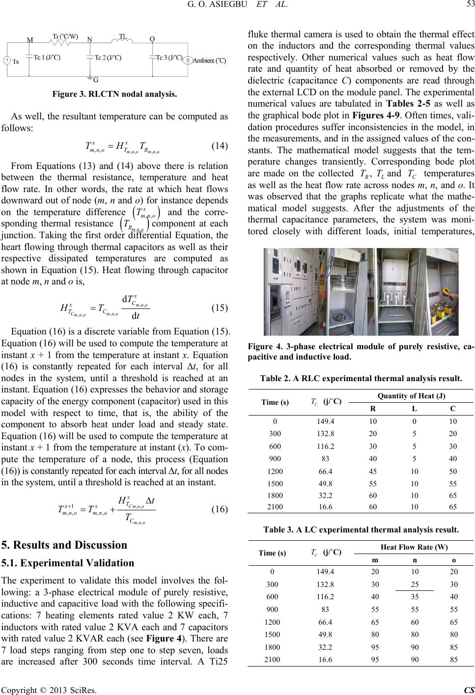

G. O. ASIEGBU ET AL. 53
Figure 3. RLCTN nodal analysis.
As well, the resultant temperature can be computed as
follows:
,, ,,mno mno
xx
T R
THT

,,
x
mn
T
,,
mno (14)
From Equations (13) and (14) above there is relation
between the thermal resistance, temperature and heat
flow rate. In other words, the rate at which heat flows
downward out of node (m, n and o) for instance depends
on the temperature difference o and the corre-
sponding thermal resistance


T,,mno
Rcomponent at each
junction. Taking the first order differential Equation, the
heart flowing through thermal capacitors as well as their
respective dissipated temperatures are computed as
shown in Equation (15). Heat flowing through capacitor
at node m, n and o is,
,,
,,
d
d
mno
Cmno
x
C
TC
T
t
,,mno
x
HT (15)
Equation (16) is a discrete variable from Equation (15).
Equation (16) will be used to compute the temperature at
instant x + 1 from the temperature at instant x. Equation
(16) is constantly repeated for each interval ∆t, for all
nodes in the system, until a threshold is reached at an
instant. Equation (16) expresses the behavior and storage
capacity of the energy component (capacitor) used in this
model with respect to time, that is, the ability of the
component to absorb heat under load and steady state.
Equation (16) will be used to compute the temperature at
instant x + 1 from the temperature at instant (x). To com-
pute the temperature of a node, this process (Equation
(16)) is constantly repeated for each interval ∆t, for all nodes
in the system, until a threshold is reached at an instant.
,,
,,
Cm n o
mno
x
T
oC
1
,, ,,
xx
mno mn
H
t
T


,
TT
 (16)
5. Results and Discussion
5.1. Experimental Validation
The experiment to validate this model involves the fol-
lowing: a 3-phase electrical module of purely resistive,
inductive and capacitive load with the following specifi-
cations: 7 heating elements rated value 2 KW each, 7
inductors with rated value 2 KVA each and 7 capacitors
with rated value 2 KVAR each (see Figure 4). There are
7 load steps ranging from step one to step seven, loads
are increased after 300 seconds time interval. A Ti25
fluke thermal camera is used to obtain the thermal effect
on the inductors and the corresponding thermal values
respectively. Other numerical values such as heat flow
rate and quantity of heat absorbed or removed by the
dielectric (capacitance C) components are read through
the external LCD on the module panel. The experimental
numerical values are tabulated in Tables 2-5 as well as
the graphical bode plot in Figures 4-9. Often times, vali-
dation procedures suffer inconsistencies in the model, in
the measurements, and in the assigned values of the con-
stants. The mathematical model suggests that the tem-
perature changes transiently. Corresponding bode plot
are made on the collected
R
Land C temperatures
as well as the heat flow rate across nodes m, n, and o. It
was observed that the graphs replicate what the mathe-
matical model suggests. After the adjustments of the
thermal capacitance parameters, the system was moni-
tored closely with different loads, initial temperatures,
TT T
Figure 4. 3-phase electrical module of purely resistive, ca-
pacitive and inductive load.
Table 2. A RLC experimental thermal analysis result.
Quantity of Heat (J )
Time (s) C
T (j/˚C) R L C
0 149.4 10 0 10
300 132.8 20 5 20
600 116.2 30 5 30
900 83 40 5 40
1200 66.4 45 10 50
1500 49.8 55 10 55
1800 32.2 60 10 65
2100 16.6 60 10 65
Table 3. A LC experimental thermal analysis result.
Heat Flow Rate (W)
Time (s) C
T (j/˚C) m n o
0 149.4 20 10 20
300 132.8 30 25 30
600 116.2 40 35 40
900 83 55 55 55
1200 66.4 65 60 65
1500 49.8 80 80 80
1800 32.2 95 90 85
2100 16.6 95 90 85

G. O. ASIEGBU ET AL.
54
Table 4. A LC experimental thermal analysis result.
Quantity of Heat (J )
Time (s) C
T (j/˚C) R L C
0 149.4 0 0 0
300 132.8 1 10 10
600 116.2 1 10 10
900 83 1 10 10
1200 66.4 2 20 20
1500 49.8 2 20 20
1800 32.2 2 20 20
2100 16.6 3 30 20
Table 5. A RL experimental thermal analysis result.
Quantity of Heat (J )
Time (s) C
T (j/˚C) R L C
0 149.4 20 30 3
300 132.8 40 60 5
600 116.2 90 60 8
900 83 80 120 11
1200 66.4 90 150 13
1500 49.8 110 180 15
1800 32.2 130 200 18
2100 16.6 130 200 21
Figure 5. Effect of heat absorbed by dielectric


C
T

R
T
and
core on the winding.
Figure 6. Heat flow rate across nodes m, n, o in the
RLCTN.
different time intervals and different environment condi-
tions. All the validations were much similar to the mathe-
matical model.

Figure 7. Effect of insufficient thermal resistance

R
T on
the winding


L.
Figure 8. Effect of thermal capacitance degradation on
the winding
C
T


L.
Figure 9. Thermal gradient with respect to time at
. C,C

498J14 kWand14
CR L
TT T

T
.
The experimental values in Table 2 show the effect of
varying the thermal capacitance on the RLC components,
the higher thermal capacitance value the lower heat dis-
sipation on the RLCTN components and vice vase. More
explanation about this is graphically illustrated in Figure
5. This Figure shows the effect of quantity of heat ab-
sorbed by the dielectric (C) components on winding (L).
As defined in Section 2, the combination of thermal
components: the dielectric materials

Cand the core


R
T resulted in logarithmic drop of winding tempera-
ture


L
T. Hence, more heat is been radiated to the am-
bient through the transformer radiator as illustrated in
Figure 2.

G. O. ASIEGBU ET AL. 55
The values in Table 3 also show the effect of varying
thermal capacitance on the thermal nodes (m, n, and o) as
shown in Figure 3. This explains the higher thermal ca-
pacitance the slower heat flow rate to the node junc-
tions and vice vase. In the case transformers, this reduces
the risk of arc flash between phases or phase and neutral
[19-21]. Figure 6 replicates the nodal analysis method
well defined in Section 3 and thermal equivalent of Kir-
chhoff’s Law, stating that temperature difference be-
tween any two points has to be independent of the path
used to travel between the two points. Figure 6 graphi-
cally illustrates that the heat flow rate across the nodes
were linearly increased and stabilized at about 1750 sec
time interval.
In Table 4, it is seen that there was insufficient ther-
mal resistance

R
T
C
T

T

T
which represent the transformer
core. Here it was observed that the transformer winding
(L) temperature increased to about 30˚C irrespective of
the high thermal capacitance value

. Figure 7
shows the graphical illustration.
The experimental value in Table 5 shows the effect of
thermal capacitance C degradation, which represents
the dielectrics of a transformer such as oil. Here also it is
seen that the transformer dielectric Cmaterials have
decreased in its heat absorption capacity causing the
winding temperature to rise so high up to 180˚C at
1500 sec irrespective of the high thermal resistance value

L
R
T

C
. Figure 8 graphically show the effect of thermal ca-
pacitance degradation.

T
5.2. Verification of Simulation
The RLCTN was simulated with Multisim software in
order to verify the results of the experiment performed in
the power system laboratory using RLC electrical mod-
ule and thermal imager. Comparing Figures 9-11 it is
obvious that the lager the thermal capacitance slower the
transient response time that is, the rate at which tem-
perature rises is much slower and vice vase. With refer-
ence to the model in Figure 2, the effect of RLC pa-
rameters used are considered with three different values
of thermal capacitance at constant thermal resistance and
thermal inductance values: 49.8 J/˚C, 199.2 J/˚C, 348.6
J/˚C and 14 k˚C/W and 14
L
T for thermal capacitance
of transformer components for instance winding, core, oil
and radiator. For this simulation, there are set initial con-
ditions namely, the winding temperature = 38˚C, the core
surface temperature = 25˚C, the oil temperature = 15˚C
and radiator temperature = 8˚C. These mentioned schemes
shows the rate of temperature rise of an oil transformer
that means the higher the thermal capacitance the slower
the rate of temperature rise. In other words, the capacity
of the oil and radiators to absorb heat emitted by the
winding and core depends on the dielectric property such
as volume, type of material, air space, and other proper-
ties. In these scenarios, the time constant (i.e., the time it
takes for the transformer winding to achieve its highest
stable temperature) changes from 0 second to 10 seconds
as shown in Figures 9-11, respectively, even though the
final temperature is the same. Statistically, in consumer
or industrial applications, a transformer temperature rise
of about 40˚C to 50˚C may be acceptable, resulting in a
maximum internal temperature of about 100˚C (trans-
formers’ temperature rise limit). However, it may be
wiser to increase the capacitance as well as the core size
in other to obtain reduced temperature rise and reduced
losses for better power supply efficiency.
Figure 10. Thermal gradient with respect to time at
C, C

199.2J14kWand14
CR L
TT T.
Figure 11. Thermal Gradient with respect to time at
C, C

348.6J14kW and14
CR L
TT T.
Figure 12. IRT color gradient of 7 transformers depicting

G. O. ASIEGBU ET AL.
56
gradual degradation of dielectric materials .

C
T
5.3. Thermal Gradient
An analytical IRT thermography is characterized with a
thermogram showing visible spectrum image, as indi-
cated in Figure 12. As stated in Section 3, thermal im-
ages of pure inductive load were captured from real time
operating transformers during validation process. This
shows the effect of dielectric failure (thermal capacitance
fault) on transformers. It was observed that as the ther-
mal capacitance value is decreasing, the transformer
temperature increase and vice vase. The color gradients
of the IRT image in Figure 12 depict severity of dielec-
tric abnormal condition that is thermal capacitance fault.
This also shows how suitable dielectric materials can
improve efficiency transformers by removing substantial
amount of heat emitted by winding and core to the am-
bient through the transformer radiators.
6. Conclusion
In this paper, a mathematical model capable of describe-
ing thermal characteristics of oil transformer was pre-
sented. The model can adequately represent thermal cha-
racterristics of each component in the transformer under
load, steady state operation, and abnormality in the di-
electric components such as the transformer oil, cellulose
insulator, and other peripherals. This model is simple,
accurate and easy to be applied for measuring the thermal
impact on transformer. It provides an easy way of pre-
dicting transformer’s thermal status. So, it allows me-
chanisms like thermal throttling and load balancing to be
more dynamic, rather than merely reacting to the situa-
tion when the temperature reach a critical point. Fur-
thermore, the algorithm is efficient enough to allow dy-
namic recomputation of the transformer temperatures
during operation. The captured thermal image brings the
qualitative thermal image analysis of the model showing
the thermal effect of gradual degradation of dielectric
materials been represented as thermal capacitance


TC
in the RLCTN. Within the limits of experimental errors,
it was observed that the RLCTN model effectively ana-
lyzed the thermal degradation of transformer dielectrics
with respect to time. Also the mathematical results repli-
cate the simulation and experimental results, as it showed
that thermal capacitance of dielectrics is inversely pro-
portional to the transformer thermal rise.
REFERENCES
[1] D. Susa, M. Lehtonen and H. Nordman, “Dynamic Ther-
mal Modeling of Distribution Transformers,” IEEE Trans-
actions on Power Delivery, Vol. 20, No. 3, 2005, pp
1919-1929.
http://www.ndted.org/EducationResources/CommunityCo
llege/Other%20Methods/IRT/IR_Applications.htm
[2] M. Matian, A. J. Marquis and N. P. Brandon, “Applica-
tion of Thermal Imaging to Validate a Heat Transfer
Model for Polymer Electrolyte Fuel Cells,” International
Journal of Hydrogen Energy, Vol. 35, No. 22, 2010, pp
12308-12316. doi:10.1016/j.ijhydene.2010.08.041
[3] Infraspection Institute, “Standard for Infrared Inspection
of Electrical Systems & Rotating Equipment,” In: Infras-
pection Institute, Infrared Training and Infrared Certifi-
cation, Infraspection Institute, Burlington, 2008.
[4] T. M. Lindquist, L. Bertling and R. Eriksson, “Estimation
of Disconnectors Contact Condition for Modeling the Ef-
fect of Maintenance and Ageing,” Power Tech IEEE
Conference, St. Petersburg, 27-30 June 2005, pp. 1-7.
[5] N. Rada, G. Triplett, S. Graham and S. Kovaleski,
“High-Speed Thermal Analysis of High Power Diode
Arrays,” Solid-State Electronics ISDRS, Vol. 52, No. 10,
2008, pp. 1602-1605. doi:10.1016/j.sse.2008.06.009
[6] Y. Cao, X. M. Gu and Q. Jin, “Infrared Technology in the
Fault Diagnosis of Substation Equipment,” China Inter-
national Conference on Electricity Distribution, Guang-
zhou, 10-13 December 2008, pp. 1-6.
[7] A. M. A. Haidar, G. O. Asiegbu, K. Hawari and F. A. F.
Ibrahim, “Electrical Defect Detection in Thermal Image,”
Advanced Materials Research, Vol. 433-440, 2012, pp
3366-3370.
[8] Y. Cao, X. M. Gu and Qi Jin, “Infrared Technology in the
Fault Diagnosis of Substation Equipment,” Technical
Session 1 Distribution Network Equipment, Shanghai
Electric Power Company Shanghai Branch Southern
Power, 200030, SI-17 CP1377, CICED2008.
[9] J. G. Smith, B Venkoba Rao, V. Diwanji and S. Kamat,
“Fault Diagnosis—Solation of Malfunctions in Power
Transformers,” Tata Consultancy Services Limited, Vol.
10, No. 1, 2009, pp. 1-12.
[10] R. M. Button, “Soft-Fault Detection Technologies De-
veloped for Electrical Power Systems,” 2005.
http://powerweb.grc.nasa.gov/elecsys/
[11] Martin Technical Electrical Safety & Efficiency, “Infra-
red Thermography Inspection,” 2012.
http://www.martechnical.com/infrared_inspections/electri
cal_infrared_inspection_service.php
[12] G. Biswas, R. Kapadia, D. Xu and W. Yu, “Combined
Qualitative—Quantitative Steady-State Diagnosis of Con-
tinuous-Valued Systems,” IEEE Transactions on Systems,
Man, and Cybernetics—Part A: Systems and Humans,
Vol. 27, No. 2, 1997, pp. 167-185.
doi:10.1109/3468.554680
[13] N. Radaa, G. Tripletta and S. Graham, “High-Speed
Thermal Analysis of High Power Diode Arrays,” Solid-
State Electronics ISDRS, College Park, 12-14 December
2007.
[14] K. C. P. Wong, H. M. Ryan and J. Tindle, “Power System
Fault Prediction Using Artificial Neural Networks,” In-
ternational Conference on Neural Information Processing,
Hong Kong, 24-27 September 1996, Article ID: 17762.

G. O. ASIEGBU ET AL.
57
[15] M. S. Jadin, S. Taib, S. Kabir and M. A. B. Yusof, “Im-
age Processing Methods for Evaluating Infrared Thermo-
graphic Image of Electrical Equipment,” Progress in
Electromagnetics Research Symposium Proceedings,
Marrakesh, 20-23 March 2011, p. 1299.
[16] Electric Power Engineering Center “Guide to Power
Transformer Specification Issues,” University of Canter-
bury, 2007.
http://www.scribd.com/doc/65031914/EPECentre-Guide-
to-Transformer-Specification-Issues
[17] K. Harwood, “Modeling a RLC Circuit’s Current with
Differential Equations,” 2011.
http://home2.fvcc.edu/~dhicketh/DiffEqns/Spring11proje
cts/Kenny_Harwood/ACT7/KennyHarwoodFinalProject.
pdf
[18] A. P. Ferreira, D. Mossé and J. C. Oh, “Thermal Faults
Modeling Using a RC Model with an Application to Web
Farms,” 19th Euromicro Conference on Real-Time Sys-
tems (ECRTS 07), Pisa, 4-6 July 2007, pp. 113-124.
[19] M. Holt, “Understand the National Electricity Codes,”
Cengage Learning, Delmar, 2002.
[20] R. W. Hurst, “Electrical Safety and Arc Flash Hand-
book,” Vol. 6, Electricity Forum, 2007.
http://www.meisterintl.com/PDFs/Electrical-Safety-Arc-F
lash-Handbook-Vol-5.pdf
[21] T. Crnko and S. Dyrnes, “Arcing Flash/Blast Review with
Safety Suggestions for Design and Maintenance,” Pro-
ceeding of the IEEE conference on Industry Technical,
Atlanta, 19-23 June 2000, pp. 118-126.
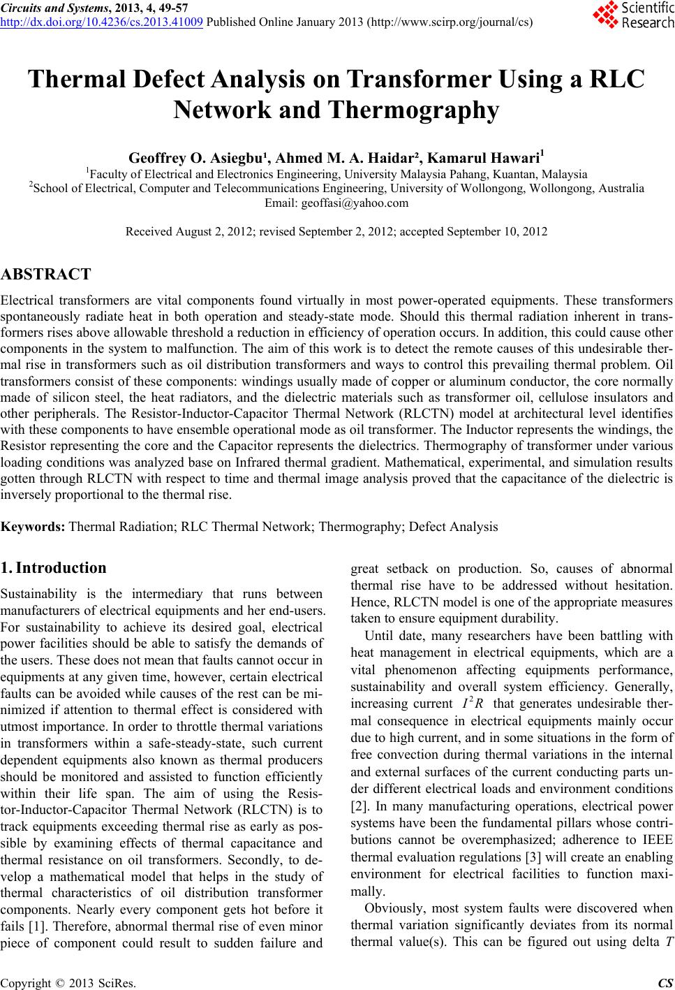