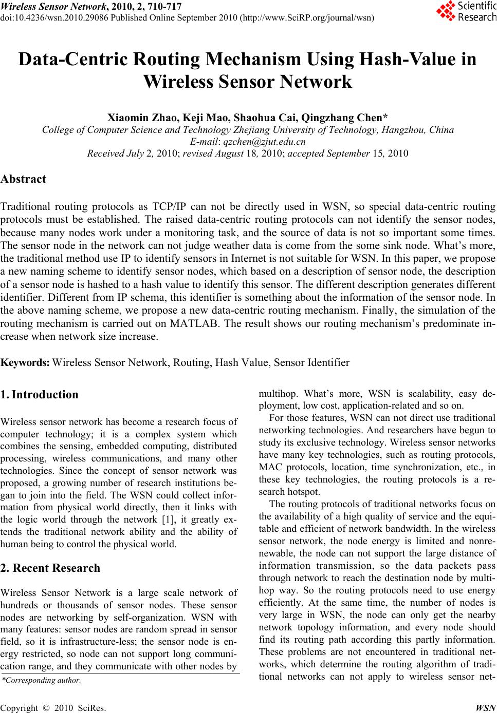Wireless Sensor Network, 2010, 2, 710-717
doi:10.4236/wsn.2010.29086 Published Online September 2010 (http://www.SciRP.org/journal/wsn)
Data-Centric Routing Mechanism Using Hash-Value in
Wireless Sensor Network
Xiaomin Zhao, Keji Mao, Shaohua Cai, Qingzhang Chen*
College of Computer Science and Technology Zhejiang University of Technology, Hangzhou, China
Received July 2, 2010; revised August 18, 2010; accepted September 15, 2010
Abstract
Traditional routing protocols as TCP/IP can not be directly used in WSN, so special data-centric routing
protocols must be established. The raised data-centric routing protocols can not identify the sensor nodes,
because many nodes work under a monitoring task, and the source of data is not so important some times.
The sensor node in the network can not judge weather data is come from the some sink node. What’s more,
the traditional method use IP to identify sensors in Internet is not suitable for WSN. In this paper, we propose
a new naming scheme to identify sensor nodes, which based on a description of sensor node, the description
of a sensor node is hashed to a hash value to identify this sensor. The different description generates different
identifier. Different from IP schema, this identifier is something about the information of the sensor node. In
the above naming scheme, we propose a new data-centric routing mechanism. Finally, the simulation of the
routing mechanism is carried out on MATLAB. The result shows our routing mechanism’s predominate in-
crease when network size increase.
Keywords: Wireless Sensor Network, Routing, Hash Value, Sensor Identifier
1. Introduction
Wireless sensor network has become a research focus of
computer technology; it is a complex system which
combines the sensing, embedded computing, distributed
processing, wireless communications, and many other
technologies. Since the concept of sensor network was
proposed, a growing number of research institutions be-
gan to join into the field. The WSN could collect infor-
mation from physical world directly, then it links with
the logic world through the network [1], it greatly ex-
tends the traditional network ability and the ability of
human being to control the physical world.
2. Recent Research
Wireless Sensor Network is a large scale network of
hundreds or thousands of sensor nodes. These sensor
nodes are networking by self-organization. WSN with
many features: sensor nodes are random spread in sensor
field, so it is infrastructure-less; the sensor node is en-
ergy restricted, so node can not support long communi-
cation range, and they communicate with other nodes by
multihop. What’s more, WSN is scalability, easy de-
ployment, low cost, application-related and so on.
For those features, WSN can not direct use traditional
networking technologies. And researchers have begun to
study its exclusive techno logy. Wireless sensor networks
have many key technologies, such as routing protocols,
MAC protocols, location, time synchronization, etc., in
these key technologies, the routing protocols is a re-
search hotspot.
The routing protocols of traditional networks focus on
the availability of a high quality of service and the equi-
table and efficient of network bandwid th. In the wireless
sensor network, the node energy is limited and nonre-
newable, the node can not support the large distance of
information transmission, so the data packets pass
through network to reach the destination node by multi-
hop way. So the routing protocols need to use energy
efficiently. At the same time, the number of nodes is
very large in WSN, the node can only get the nearby
network topology information, and every node should
find its routing path according this partly information.
These problems are not encountered in traditional net-
works, which determine the routing algorithm of tradi-
tional networks can not apply to wireless sensor net-
*Corresponding author.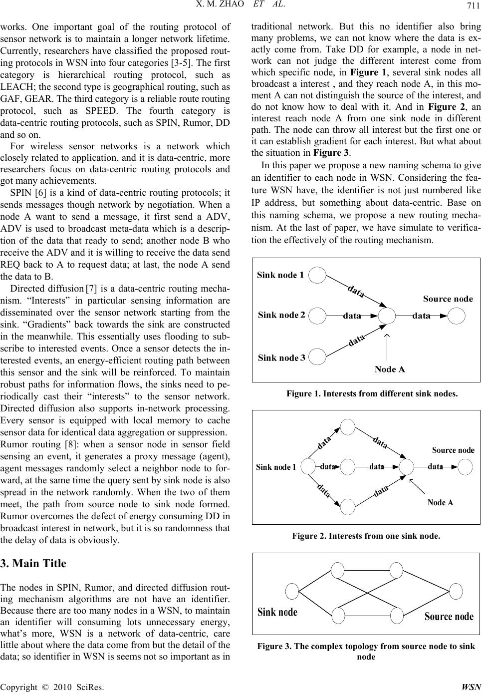

X. M. ZHAO ET AL.
711
works. One important goal of the routing protocol of
sensor network is to maintain a longer network lifetime.
Currently, researchers have classified the proposed rout-
ing protocols in WSN into four categories [3-5]. The first
category is hierarchical routing protocol, such as
LEACH; the second type is geograp h ical routin g, su ch as
GAF, GEAR. The third category is a reliable route routi ng
protocol, such as SPEED. The fourth category is
data-centric routing protocols, such as SPIN, Rumor, DD
and so on.
For wireless sensor networks is a network which
closely related to application, and it is data-cen tric, more
researchers focus on data-centric routing protocols and
got many achievements.
SPIN [6] is a kind of data-centric routing protocols; it
sends messages though network by negotiation. When a
node A want to send a message, it first send a ADV,
ADV is used to broadcast meta-data which is a descrip-
tion of the data that ready to send; another node B who
receive the ADV and it is willing to receive the data send
REQ back to A to request data; at last, the node A send
the data to B.
Directed diffusion [7] is a data-centric routing mecha-
nism. “Interests” in particular sensing information are
disseminated over the sensor network starting from the
sink. “Gradients” back towards the sink are constructed
in the meanwhile. This essentially uses flooding to sub-
scribe to interested events. Once a sensor detects the in-
terested events, an energy-efficient routing path between
this sensor and the sink will be reinforced. To maintain
robust paths for information flows, the sinks need to pe-
riodically cast their “interests” to the sensor network.
Directed diffusion also supports in-network processing.
Every sensor is equipped with local memory to cache
sensor data for identical data aggregatio n or suppression.
Rumor routing [8]: when a sensor node in sensor field
sensing an event, it generates a proxy message (agent),
agent messages randomly select a neighbor node to for-
ward, at the same time the query sent by sink node is also
spread in the network randomly. When the two of them
meet, the path from source node to sink node formed.
Rumor overcomes the defect of energy consuming DD in
broadcast interest in network, but it is so rando mness that
the delay of data is obviously.
3. Main Title
The nodes in SPIN, Rumor, and directed diffusion rout-
ing mechanism algorithms are not have an identifier.
Because there are too many nodes in a WSN, to maintain
an identifier will consuming lots unnecessary energy,
what’s more, WSN is a network of data-centric, care
little about where the data come from but the detail of the
data; so identifier in WSN is seems not so important as in
traditional network. But this no identifier also bring
many problems, we can not know where the data is ex-
actly come from. Take DD for example, a node in net-
work can not judge the different interest come from
which specific node, in Figure 1, several sink nodes all
broadcast a interest , and they reach node A, in this mo-
ment A can not distinguish the source of the interest, and
do not know how to deal with it. And in Figure 2, an
interest reach node A from one sink node in different
path. The node can throw all interest but the first one or
it can establish gradient for each interest. But what abo ut
the situation in Figure 3.
In this paper we propose a new naming schema to give
an identifier to each node in WSN. Considering the fea-
ture WSN have, the identifier is not just numbered like
IP address, but something about data-centric. Base on
this naming schema, we propose a new routing mecha-
nism. At the last of paper, we have simulate to verifica-
tion the effectively of th e routing mechanism.
Figure 1. Interests from different sink nodes.
Figure 2. Interests from one sink node.
Figure 3. The complex topology from source node to sink
node

X. M ZHAO ET AL.
712
4. Naming Scheme Based on Hash Value
Paper [9,10] proposed a data-centric storage scheme, use
data itself to describe its storage location, that is the
name of the data represent a keyword, you can use this
keyword to find the data. And queries can be routed to
the data directly by the name of the corresponding node.
In this paper, we propose a new naming scheme accord-
ing to data-centric scheme above. We first describe the
data by attribute pairs, for example: there is a sensor
node in the room 621 of library to monitor the tempera-
ture, and then it has a description below:
ATTRIBUTION{
Service = temperature
Room = R621
Building = library
} (1)
If the node has more than one sensor model, performs
several monitor task, for example the sensor node in
room 621 not only monitor the temperature but also ob-
ject monitor, then it can also describe like this:
ATTRIBUTION{
Service = Object Monitor
Room = R621
Building = library
} (2)
One node could have several descriptions, but one de-
scription can only describe one node.
Meanwhile, we use the same naming scheme to name
the query, such as a query to check the room 621’s tem-
perature, and then the description of this query is:
ATTRIBUTION{
Service = temperature
Room = R621
Building = library
} (3)
After each node and query has its description, we use a
certain hash algorithm to generate a hash value, and use
this hash value to identify the node or query. For the
above description (1) and (3), (1) describes the detail of
node in room 621 and (3) describes the query whose des-
tination is node in room621. We can find that the de-
scription of (1) and (3) is identical; by the same hash
function the query will generate the same hash value
with its destination node. So it can be routed directly and
correctly. Thus each node in network will have a unique
identifier.
According to this naming scheme, we can map the
complex physical topology of a network to one-dimen-
sional logical topology. As shown in Figure 4. One node
could have several ID to identify itself, for example v6
mapped to a3 and a6, but one ID can unique identify a
node.
Figure 4. Mapping from physical topology to logical topol-
ogy.
This naming scheme based on hash value is aiming to
solve the problems in raised data-centric routing mecha-
nism which has no uniform identification. And this
naming scheme is different from the traditional network
which base on IP address, the ID of node is not just a
number, but a keyword of data, it is data-centric.
5. Routing Mechanism
Base on the above naming schema, each node maintains
a routing table, a logical neighbor table and a physical
neighbor table, and according to those routing informa-
tion, messages can be delivered to destination efficiently.
5.1. Tables of Routing Information
5.1.1. Routin g Table
Routing table is used to help messages to deliver to des-
tination, it maintains three paramet ers. The first parame ter
is leader node, leader nodes are those identifying
hash-value that closest to R/2n away from the hash value
of local sensor, while R as the range of the hash domain,
and n is the routing scope. The second parameter is path,
it record the path to the leader and the third parameter is
cost it spends from local node to leader. Figure 5 is the
structure of the routing table.
For one node, there are several scopes about leader.
The first scope is the node whose ID is closest to R/2,
and the second scope is the node whose ID is closest to
R/4, and third scope R/8…, we select leader by the for-
mula below:
2
nn
R
Uv
“n” is the scope of leader. So, node v0’s namespace can
be segmented as in Figure 6.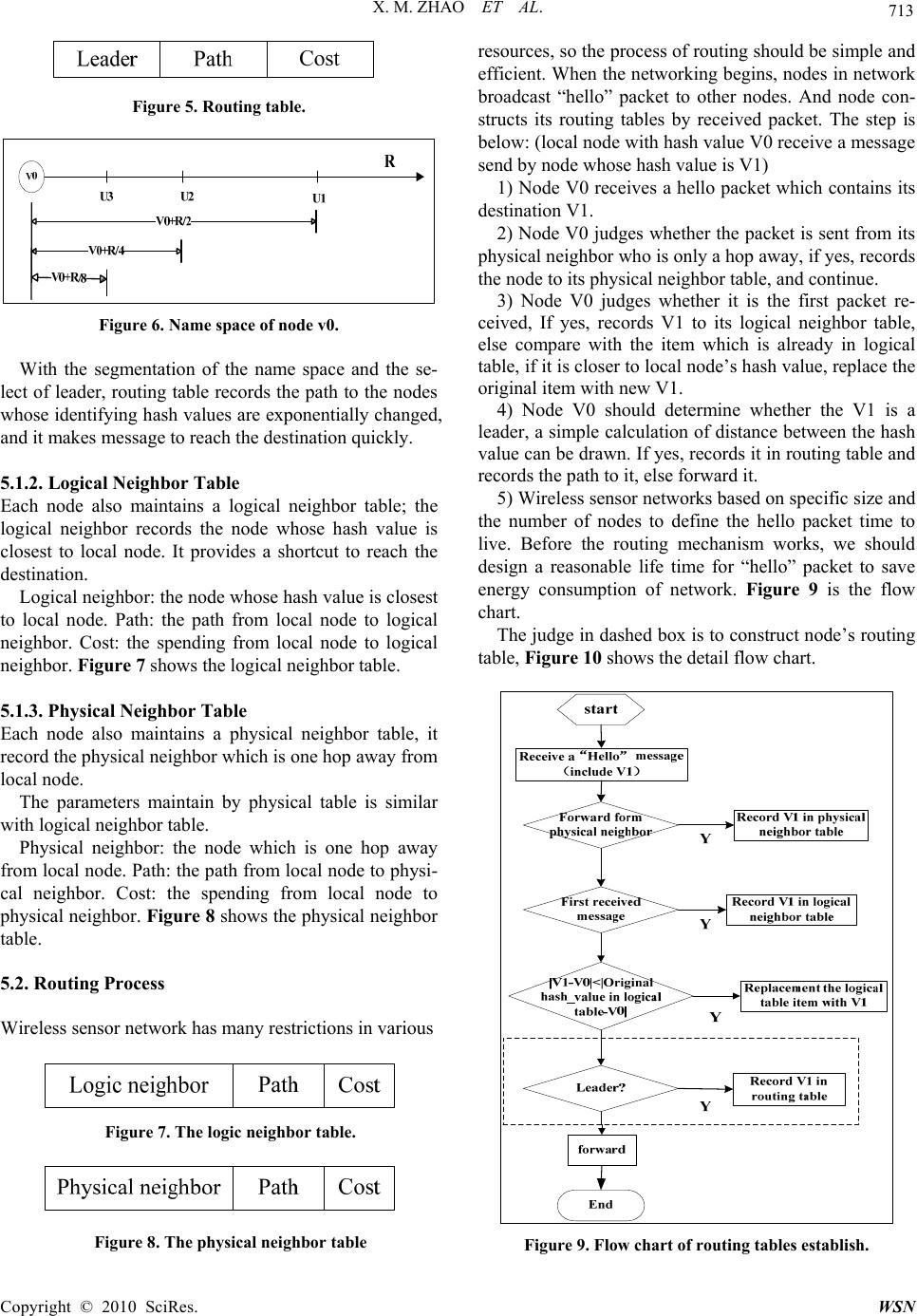

X. M. ZHAO ET AL.
713
Figure 5. Routing table.
Figure 6. Name space of node v0.
With the segmentation of the name space and the se-
lect of leader, routing table records the path to the nodes
whose identifying hash values are exponentially changed,
and it makes message to reach the destination quickly.
5.1.2. Logical Neighbor Table
Each node also maintains a logical neighbor table; the
logical neighbor records the node whose hash value is
closest to local node. It provides a shortcut to reach the
destination.
Logical neighbor: the node whose hash value is closest
to local node. Path: the path from local node to logical
neighbor. Cost: the spending from local node to logical
neighbor. Figure 7 shows the logical neighbor table.
5.1.3. Physical Neighbor Table
Each node also maintains a physical neighbor table, it
record the physical neighbor which is one hop away from
local node.
The parameters maintain by physical table is similar
with logical neighbor table.
Physical neighbor: the node which is one hop away
from local node. Path: the path from local node to physi-
cal neighbor. Cost: the spending from local node to
physical neighbor. Figure 8 shows the ph ysical neighbor
table.
5.2. Routing Process
Wireless sensor net w or k has m a ny restrict i o ns i n vario us
Figure 7. The logic neighbor table.
Figure 8. The physical neighbor table
resources, so the process of routing should be simple and
efficient. When the networking begins, nodes in network
broadcast “hello” packet to other nodes. And node con-
structs its routing tables by received packet. The step is
below: (local node with hash value V0 receive a message
send by node whose hash value is V1)
1) Node V0 receives a hello packet which contains its
destination V1.
2) Node V0 judges whether the packet is sent from its
physical neighbor who is on ly a hop away, if yes, records
the node to its physical neighbor table, and continue.
3) Node V0 judges whether it is the first packet re-
ceived, If yes, records V1 to its logical neighbor table,
else compare with the item which is already in logical
table, if it is closer to local node’s hash value, replace the
original item with new V1.
4) Node V0 should determine whether the V1 is a
leader, a simple calculation of distance between the hash
value can be drawn. If yes, records it in routing table and
records the path to it, else forward it.
5) Wireless sensor networks based on specific size and
the number of nodes to define the hello packet time to
live. Before the routing mechanism works, we should
design a reasonable life time for “hello” packet to save
energy consumption of network. Figure 9 is the flow
chart.
The judge in dashed box is to construct node’s rou ting
table, Figure 10 shows the detail flow chart.
Figure 9. Flow chart of routing tables establish.

X. M ZHAO ET AL.
714
star t
“Hello” message
(include V 1)
V1-V0=R/2
V1-V0=R/4
V1-V0=R/8
R ecord V 1 as 1st
leader
Re c o r d V1 as 2 n d
leader
R eco rd V1 a s 3th
leader
end
forward
……
Y
Y
Y
Figure 10. Flow chart of leader definite.
With the three tables of routing information, the node
can forward every packet wherever its destination is. The
routing mechanism as:
1) When a node receives a packet from other node, it
first checks its physical neighbor table and logical
neighbor table to determine whether there is a path to the
destination node, if yes, send the packet to node record
by either table.
2) Otherwise, the node calculate its own hash value
and the packet hash value to determine which scope of
leader the node need to help to forwar d the packet. For
example: If the packet’s hash value is closer to the 1st
leader, then it forwards the packet to its 1st leader.
3) Repeat step one, step two, until the packet accu-
rately reach its destination.
5.3. Route Maintenance
By the networking is complete, we need maintenan ce the
routing information regular to ensure the correctness.
The simplest method is to periodically broadcast the
node’s hash value contains in a “hello” packet, to declare
its own survival. If one node hasn’t broadcast a hello
packet for a long time, then other node will think it is fo r
some reasons departed from network, and the path con-
tains this node will failure.
When invalid nodes leaver or new nodes join the net-
work, the routing table and neighbor table need to be
updated.
5.3.1. New Nodes Join the Network
When a new node needs to join a network, its routing
information should be constructed first.
1) To join a sensor network, a new sensor first con-
tacts one of its “physical” neighbors randomly to con-
struct physical neighbor table. A sensor’s physical
neighbors are those sensors geographically close.
2) Then this sensor generates log 1R


joining re-
quests with a key R/2n plus its identifying hash value.
Conceptually, these jo ining requests will be forwarded to
the sensors that are numerically closest to each key. The
Sensors visited by a joining request will be recorded in
this request to track the routing path. When those re-
quests reach the destination, the destination node records
the new node and reply. After collecting all the replies,
the new sensor can construct its own routing table.
3) This sensor generates a joining request with a key of
its own identifying hash value. This joining request is
used to construct the neighbor table. When the nu merica ll y
closest sensor to that hash value receives the joining re-
quest, it returns its logical neighbors and the paths to the
neighbors to the new sensor and meanwhile updates its
neighbor table with that hash value and the routing path
recorded in the request. The reply of this reply provides
the information of node’s logical neighbor.
5.3.2. Nodes Withdraw from the Network
Wireless sensor network is a kind of dynamic, adaptive
network, if a node’s energy is exhaust, or for other rea-
sons lost its contact with the network. So the routing in-
formation is not correctness, to supp ort robustness of the
sensor network, the sensors need to update the routing
tables periodically.
5.3.3. Support for Mobile Node
Although most of the nodes in wireless sensor network
are fixed, there is a part of node need mobility, and those
nodes always play an important role. How to support
mobile nodes properly is a new challenge in wireless
sensor network. Figure 11 shows the WSN with mobile
node A.
By the naming schema raised in paper, each nodes use
a hash value to identify themselves, so we can map the
complex physical topology into a 1-D logical topology,
as Figure 1 describe. In this case, as shown in Figure 7,
a mobile node S5, it moved from T0, T1, T2 moment,
but the hash value of S5 is changeless, so whenever the

X. M. ZHAO ET AL.
715
physical topology of the network changes, the logical
topology is changeless, shows in Figure 12, because the
identifier of the mobile node is abiding.
In this paper, we support mobile nodes by the routing
information that each nodes maintains. Firstly, we re-
quest node add an attribute to describe the node’s mobili ty.
And then we add constraints to routing tables:
1) Each node maintain a routing table, all the nodes
maintained in this table must be immovable.
2) An immovable node will maintain two different
logical neighbors, an immovable logic neighbor table
and a mobile logical neighbor table. However, the mov-
able sensor needn’t maintain a mobile logical neighbor
table.
Figure 11. Mobile nodes in WSN.
Figure 12. Mapping from physical topology to logical to-
pology with a mobile node.
3) Movable sensors also maintain an immovable logic
neighbor table and a mobile logical neighbor table. Dif-
ferent from tables immovable node maintain, it didn’t
maintain the path to neighbor node for those path is
variable.
By the constraints written above, When a mob ile node
willing to send a packet to the immovable node, it can
just forward packet to its nearest immovable physical
neighbor, and then the packet will be forwarded accord-
ing to routing mechanism. If a node has a packet to send
to the mobile node, there is no direct path to the mobile
node, the sending node will just sent it to the mobile
node's logical neighbors. Mobile node sends regular send
hello messages back to its neighbor to get the packet. In
this way, data flow from mobile node to immovable node
is established.
Here follows the concrete steps:
1) The mobile node broadcast a hello packet to other
node when reach the new place to get its physical
neighbor information.
2) When a mobile node to send a packet, it send the
packet to its physical neighbors.
3) When an immovable node has to communicate with
mobile node, either node sends packet to it or replies. It
sends the packet to mobile node’s logical neighbor.
4) The mobile node periodically sends hello packets to
its logical neighbors to get the packet.
6. Simulation
We compare proposed routing mechanism to Directed
Diffusion, Rumor, and Flooding. Figure 9 is describes
100 nodes random distribution in th e 100 meter multiply
100 meter space. Figure 13 depict node A’s logical
neighbor and leader. We can see from Figure 14 that the
logical neighbor and leader are well-proportioned in the
region. In Figure 14, red arrows point to node A’s leader,
and blue arrows point to its logical neighbor.
Figure 13. 100 nodes in 100m*100m.

X. M ZHAO ET AL.
716
The Figure 15 shows the packet number required for a
success query
Figure 14. Logical neighbor and leader of node A.
Figure 15. Packet number of a query.
Figure16. Average hops of a query.
Figure17. Average energy dissipated of a query.
The Figure 16 shows the average hops a packet cost
to destination node. From which we can see that pro-
posed routing mechanism is advantageous when the
network scale increased.
The Figure 17 is the average energy dissipated for a
discovered routing path.
7. Conclusions
The proposed routing mechanism is superior to other
data-centric routing, especially when nodes in a WSN
increased.
8. References
[1] D. Chen, Z. W. Zheng and J. J. Li, “Research on Wire le ss
Sensor Network,” Computer Measurement and Control,
Vol. 12, No. 8, 2004, pp. 701-704.
[2] L. M. Sun, “Wireless Sensor Network,” Tsinghua Uni-
versity Press, Beijing, 2005.
[3] W. Ye, J. Heidemann and D. Estrin, “An En ergy-E fficien t
MAC Protocol for Wireless Sensor Networks,” Proceed-
ings of IEEE Infocom, New York, 2002, pp. 1567-1576.
[4] W. Ye, J. Heidemann and D. Estrin, “Medium Access
Control with Coordinated Adaptive Sleeping for Wireless
Sensor Networks,” IEEE/ACM Transactions on Net-
working, Vol. 12, No. 3, December 2004, pp. 493-506.
[5] Y. Li, W. Ye and J. Heidemann, “Energy and Latency
Control in Low Duty Cycle MAC Protocols,” Proceed-
ings of the IEEE Wireless Communications and Net-
working Conference, New Orleans, March 2005, pp.
676-682.
[6] J. Kulik, W. R. Heinzelmann an d H. Balakrishna n, “Ad a p-
tive Protocols for Information Dissemination Information
in Wireless Sensor Networks,” Proceedings of the 5th
ADM/IEEE Mobicom Conference, Seattle, 1999, pp.
174-185.
[7] C. Intanagonwiwat, R. Govindan and D. Estrin, “Directed

X. M. ZHAO ET AL.
717
Diffusion: A Scalable and Robust Communication Para-
digm for Sensor Networks,” Proceedings of the 6th an-
nual international conference on Mobile computing and
networking, Boston, 2000, pp.56-67.
[8] A. Boulis, S. Ganeriwal, M. B. Srivastava, “Aggregation
in Sensor Networks: an Energy-accuracy Trade-off,”
Sensor Network Protocols and Applications, Vol. 1, No.
2, September 2003, pp. 317-331.
[9] S. Ratnasamy, B. Karp, L.Yin, F. Yu, D. Estrin, R. Go-
vindan and S. Shenker, “GHT: A Geographic Hash Table
for Data-Centric Storage,” Proceedings of the First ACM
International Workshop on Wireless Sensor Networks
and Applications, Atlanta, September 2002.
[10] S. Shenke, S. Ratnasamy, B. Karp, R. Govindan and D.
Estrin, “Data-Centric Storage in Sensornets,” ACM SIG-
COMM Computer Communication Review, Vol. 33, No.
1, January 2003, pp.137-142.