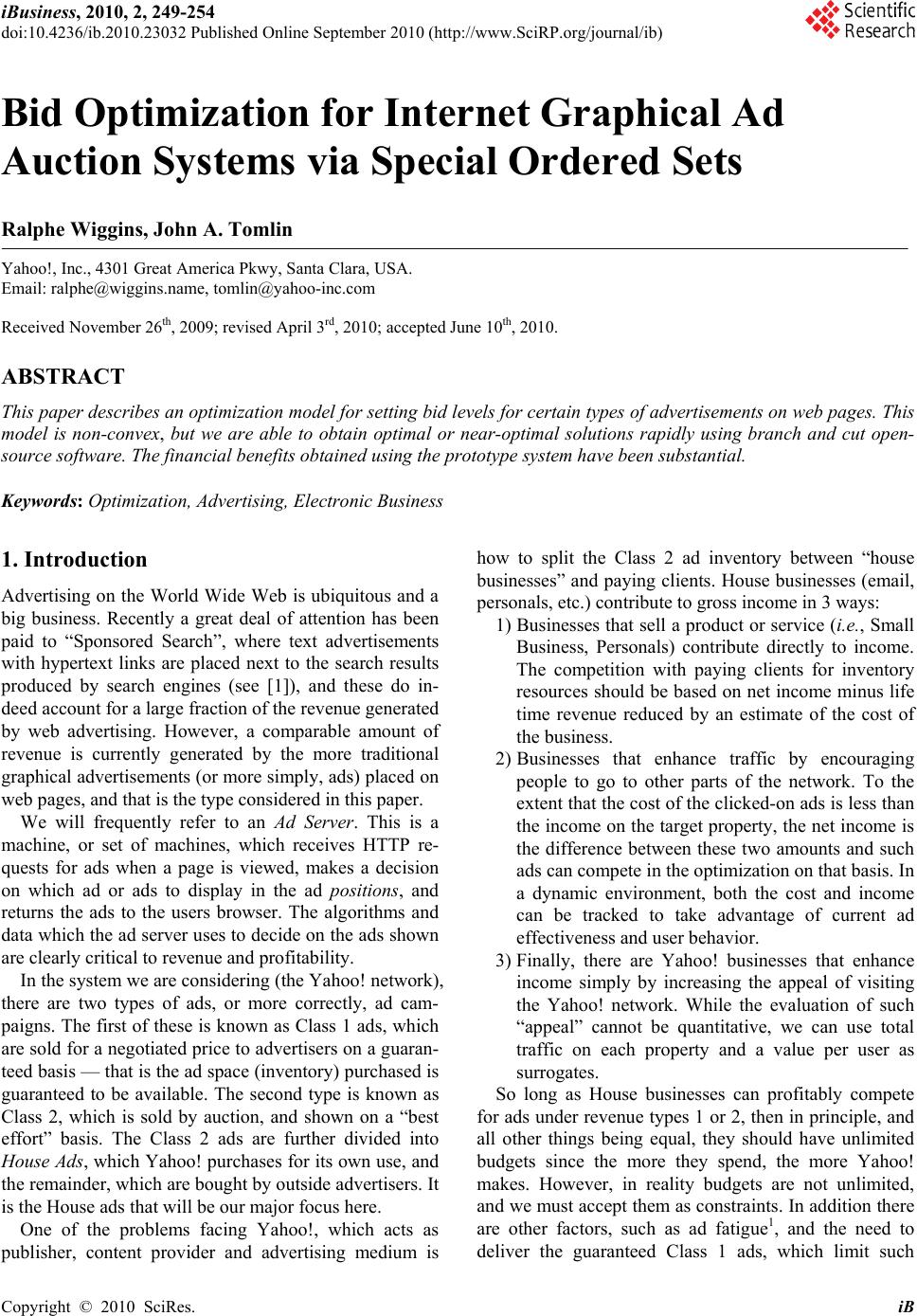iBusiness, 2010, 2, 249-254
doi:10.4236/ib.2010.23032 Published Online September 2010 (http://www.SciRP.org/journal/ib)
Bid Optimization for Internet Graphical Ad
Auction Systems via Special Ordered Sets
Ralphe Wiggins, John A. Tomlin
Yahoo!, Inc., 4301 Great America Pkwy, Santa Clara, USA.
Received November 26th, 2009; revised April 3rd, 2010; accepted June 10th, 2010.
ABSTRACT
This paper describes an optimization model for setting bid levels for certain types of advertisements on web pages. This
model is non-convex, but we are able to obtain optimal or near-optimal solutions rapidly using branch and cut open-
source software. The financial benefits obtained using the prototype system have been substantial.
Keywords: Optimization, Advertising, Electronic Business
1. Introduction
Advertising on the World Wide Web is ubiquitous and a
big business. Recently a great deal of attention has been
paid to “Sponsored Search”, where text advertisements
with hypertext links are placed next to the search results
produced by search engines (see [1]), and these do in-
deed account for a large fraction of the revenue generated
by web advertising. However, a comparable amount of
revenue is currently generated by the more traditional
graphical advertisements (or more simply, ads) placed on
web pages, and that is the type considered in this paper.
We will frequently refer to an Ad Server. This is a
machine, or set of machines, which receives HTTP re-
quests for ads when a page is viewed, makes a decision
on which ad or ads to display in the ad positions, and
returns the ads to the users browser. The algorithms and
data which the ad server uses to decide on the ads shown
are clearly critical to revenue and profitability.
In the system we are considering (the Yahoo! network),
there are two types of ads, or more correctly, ad cam-
paigns. The first of these is known as Class 1 ads, which
are sold for a negotiated price to advertisers on a guaran-
teed basis — that is the ad space (inventory) purchased is
guaranteed to be available. The second type is known as
Class 2, which is sold by auction, and shown on a “best
effort” basis. The Class 2 ads are further divided into
House Ads, which Yahoo! purchases for its own use, and
the remainder, which are bought by outside advertisers. It
is the House ads that will be our major focus here.
One of the problems facing Yahoo!, which acts as
publisher, content provider and advertising medium is
how to split the Class 2 ad inventory between “house
businesses” and paying clients. House businesses (email,
personals, etc.) contribute to gross income in 3 ways:
1) Businesses that sell a product or service (i.e., Small
Business, Personals) contribute directly to income.
The competition with paying clients for inventory
resources should be based on net income minus life
time revenue reduced by an estimate of the cost of
the business.
2) Businesses that enhance traffic by encouraging
people to go to other parts of the network. To the
extent that the cost of the clicked-on ads is less than
the income on the target property, the net income is
the difference between these two amounts and such
ads can compete in the optimization on that basis. In
a dynamic environment, both the cost and income
can be tracked to take advantage of current ad
effectiveness and user behavior.
3) Finally, there are Yahoo! businesses that enhance
income simply by increasing the appeal of visiting
the Yahoo! network. While the evaluation of such
“appeal” cannot be quantitative, we can use total
traffic on each property and a value per user as
surrogates.
So long as House businesses can profitably compete
for ads under revenue types 1 or 2, then in principle, and
all other things being equal, they should have unlimited
budgets since the more they spend, the more Yahoo!
makes. However, in reality budgets are not unlimited,
and we must accept them as constraints. In addition there
are other factors, such as ad fatigue1, and the need to
deliver the guaranteed Class 1 ads, which limit such

Bid Optimization for Internet Graphical Ad Auction Systems via Special Ordered Sets
250
Class 2 spending.
We consider setting, or rather re-setting, bids for house
Class 2 ads in such a way as to (approximately) max-
imize expected return for a large group of ads. This
involves observing the bid levels of other groups of ads
and then re-computing our bids in the relevant auctions
in such a way as to maximize expected return for the
model horiz- on. This requires choosing among discrete
bids, which can be modeled as Special Ordered Sets [2]
of type 1. A combination of heuristics applied to the LP
solution, and cutting planes, leads to rapid solution of
this discrete model.
Use of optimization models for ad campaign planning
in the presence of budgets is not completely new, either
in the traditional media (see [3]) or in the web context. In
the sponsored search setting, Abrams et al. [4] use a
linear programming model with column generation to
approach the problem. Several papers have attacked the
problem of optimizing ad serving in what we have called
the Class 1 environment (see [5] and it’s references).
However, the model discussed here has novel features
that require a different approach. The models discussed
in [5] and elsewhere assume that the model output can
specify the actual serving of specific ads for a page view,
that is dictate a serving policy to the ad server. Our only
“handle” in the Class 2 context is the bid levels to be set
for the auction procedure which then affect the serving
policy of the ad server. Clearly this implies some form of
discrete model, since a bid either exceeds another bid, or
it does not, and the outcome of that will depend on these
relative bid levels.
In the remainder of this paper we will outline some of
the terminology used with these models, discuss the data
available, formulate our model, propose some solution
strategies and give computational experience.
2. Terminology and Data
Insert order lines (IOs) correspond to the network prop-
erty/positions where an ad may be placed, i.e., a banner
ad across the top, or down the right hand (east) side of a
particular page. The number of times this position is
available (the number of impressions) is the inventory of
this IO we have available for sale.
Business lines in our context are the house businesses
seeking to buy some of this inventory. However, Class 2
inventory is sold by auction, not directly, and our only
lever to try and increase revenue for house businesses is
to set, or reset the bids for the available inventory. Since
the house is in competition with outside bidders, we need
to take those bids into account.
3. Ad Server Behavior
The ad server has quite complicated behavior. For the
purposes of this paper it is sufficient to point out that
when a request for ads from a page view arrives, a num-
ber of factors are considered. Firstly, the candidate ads
may be filtered by a user profile requested by the adver-
tiser, which must be compared with the profile of the
user (if any). Secondly, Class 1 ads will be shown in
preference to Class 2, provided that other factors such as
ad fatigue do not interfere. Finally the display of Class 2
ads is determined not only by who “wins” the auction for
this property/position, but budget limits and profile
matching. Thus the ad corresponding to the highest bid-
der is not always the one shown. When an ad (and in
particular a Class 2 ad) is shown, the appropriate budget
is decremented.
We see from this abbreviated list of characteristics that
determining the number of impressions that a Class 2 ad
will receive is not a deterministic function of the bids
alone. We are therefore reduced to approximating the
“value” of an ad with respect to its bid level by using
historical data.
4. Ad Value, Return, and Impressions
For each Insert Order Line i we define a discrete set of
bid levels ij
b, designed to just exceed the (known) com-
peting bids for the IO. A key concept in our model is the
ad value ij A associated with each bid level j for the
IO. This is our proxy for the expected amount by which
the appropriate budget will be decremented when it gets
an impression (i.e., is served up by the ad server). Asso-
ciated with this ad value is an expected total gross return
ij
L for making a bid at level j for the IO.
The number of impressions obtained will clearly be
influenced by the bid level j. Our model requires that
we have a relationship between the ad value and return
for the IO and the number of impressions expected cor-
responding to the ad values. An example of such a rela-
tionship is shown in Figure 1. The x-axis value at the
right of each horizontal segment is the expected number
of impressions received for the bid level associated with
the ad value on the y-axis. These values, denoted ij P,
along with the ij A and ij L are extrapolated from his-
torical data. Note that the actual bids ij b do not appear
themselves in the model below, and we do not discuss
the derivation of the ad values, returns, and impression
counts further in this paper.
The ad value v. impression graphs are not always as
regular as that displayed in Figure 1. More “lopsided”
examples are shown in Figures 2 and 3.
1The phenomenon whereby ads become less effective the more they are
shown to a user.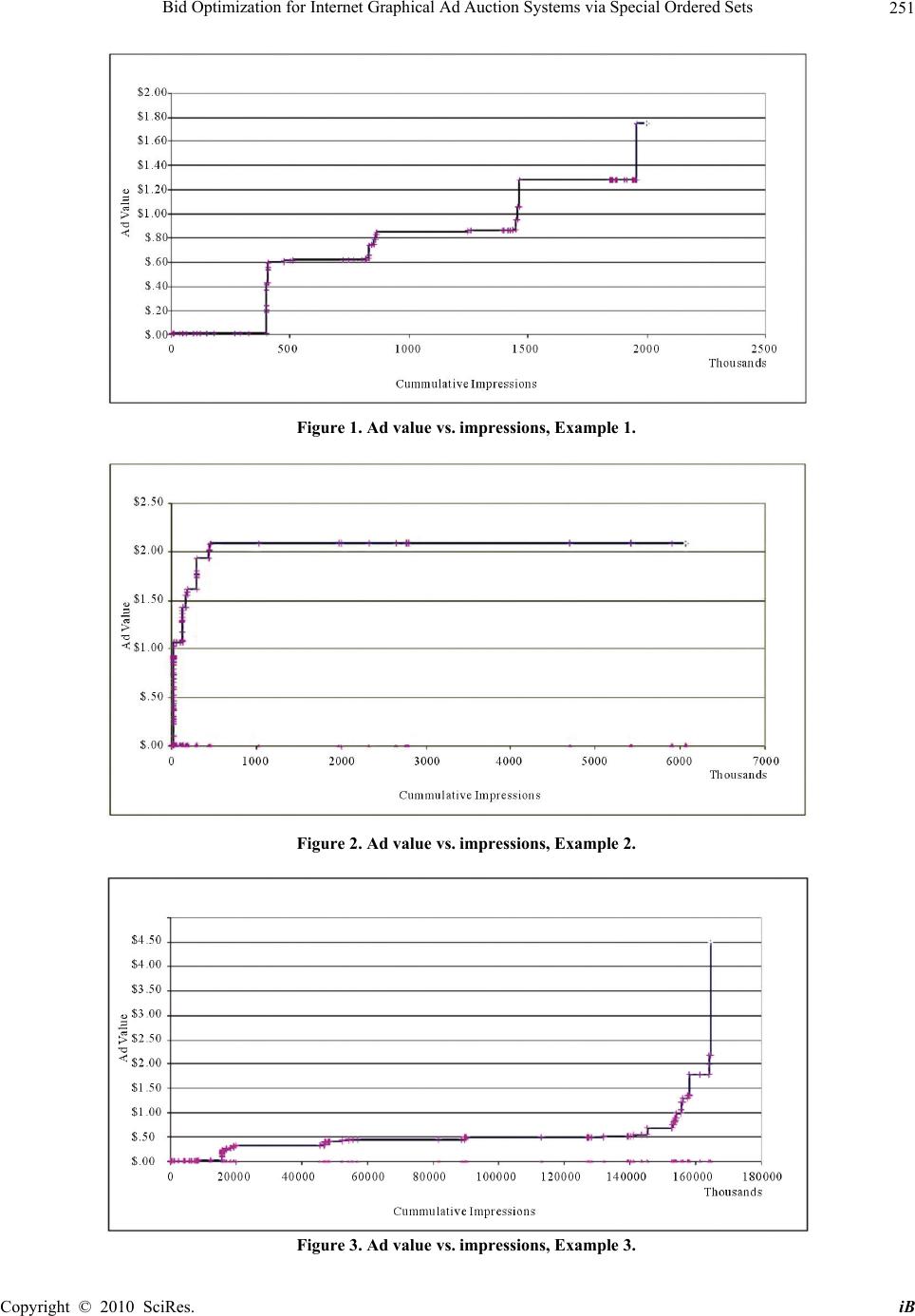

Bid Optimization for Internet Graphical Ad Auction Systems via Special Ordered Sets 251
Figure 1. Ad value vs. impressions, Example 1.
Figure 2. Ad value vs. impressions, Example 2.
Figure 3. Ad value vs. impressions, Example 3.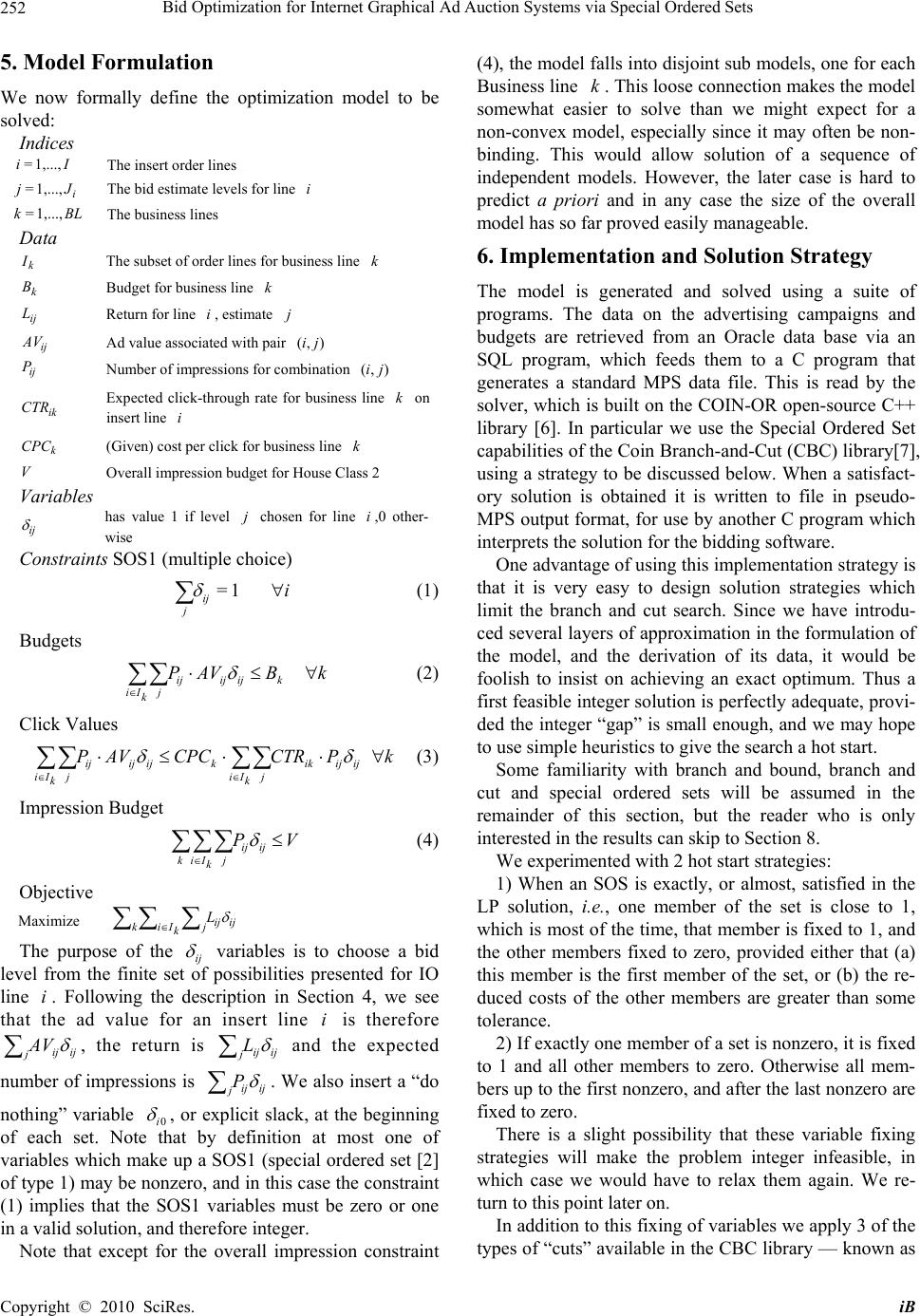

Bid Optimization for Internet Graphical Ad Auction Systems via Special Ordered Sets 252
5. Model Formulation
We now formally define the optimization model to be
solved:
Indices
Ii 1,...,= The insert order lines
i
Jj 1,...,= The bid estimate levels for line i
BLk 1,...,=
The business lines
Data
k
I The subset of order lines for business line k
k B Budget for business line k
ij L Return for line i, estimate
j
ij AV Ad value associated with pair ),( ji
ij
P
Number of impressions for combination ),(ji
ik
CTR Expected click-through rate for business line k on
insert line i
k CPC (Given) cost per click for business line k
V Overall impression budget for House Class 2
Variables
ij  has value 1 if level
j
chosen for line i,0 other-
wise
Constraints SOS1 (multiple choice)
i
ij
j

1=
 (1)
Budgets
kBAVP kijijij
j
k
Ii




(2)
Click Values
kPCTRCPCAVP ijijik
j
k
Ii
kijijij
j
k
Ii
 



 (3)
Impression Budget
VP ijij
j
k
Iik



 (4)
Objective
Maximize ijij
j
k
Iik L

 
The purpose of the ij

variables is to choose a bid
level from the finite set of possibilities presented for IO
line i. Following the description in Section 4, we see
that the ad value for an insert line i is therefore
ijij
jAV

, the return is ijij
jL

 and the expected
number of impressions is ijij
jP

. We also insert a “do
nothing” variable 0i

, or explicit slack, at the beginning
of each set. Note that by definition at most one of
variables which make up a SOS1 (special ordered set [2]
of type 1) may be nonzero, and in this case the constraint
(1) implies that the SOS1 variables must be zero or one
in a valid solution, and therefore integer.
Note that except for the overall impression constraint
(4), the model falls into disjoint sub models, one for each
Business line k. This loose connection makes the model
somewhat easier to solve than we might expect for a
non-convex model, especially since it may often be non-
binding. This would allow solution of a sequence of
independent models. However, the later case is hard to
predict a priori and in any case the size of the overall
model has so far proved easily manageable.
6. Implementation and Solution Strategy
The model is generated and solved using a suite of
programs. The data on the advertising campaigns and
budgets are retrieved from an Oracle data base via an
SQL program, which feeds them to a C program that
generates a standard MPS data file. This is read by the
solver, which is built on the COIN-OR open-source C++
library [6]. In particular we use the Special Ordered Set
capabilities of the Coin Branch-and-Cut (CBC) library[7],
using a strategy to be discussed below. When a satisfact-
ory solution is obtained it is written to file in pseudo-
MPS output format, for use by another C program which
interprets the solution for the bidding software.
One advantage of using this implementation strategy is
that it is very easy to design solution strategies which
limit the branch and cut search. Since we have introdu-
ced several layers of approximation in the formulation of
the model, and the derivation of its data, it would be
foolish to insist on achieving an exact optimum. Thus a
first feasible integer solution is perfectly adequate, provi-
ded the integer “gap” is small enough, and we may hope
to use simple heuristics to give the search a hot start.
Some familiarity with branch and bound, branch and
cut and special ordered sets will be assumed in the
remainder of this section, but the reader who is only
interested in the results can skip to Section 8.
We experimented with 2 hot start strategies:
1) When an SOS is exactly, or almost, satisfied in the
LP solution, i.e., one member of the set is close to 1,
which is most of the time, that member is fixed to 1, and
the other members fixed to zero, provided either that (a)
this member is the first member of the set, or (b) the re-
duced costs of the other members are greater than some
tolerance.
2) If exactly one member of a set is nonzero, it is fixed
to 1 and all other members to zero. Otherwise all mem-
bers up to the first nonzero, and after the last nonzero are
fixed to zero.
There is a slight possibility that these variable fixing
strategies will make the problem integer infeasible, in
which case we would have to relax them again. We re-
turn to this point later on.
In addition to this fixing of variables we apply 3 of the
types of “cuts” available in the CBC library — known as

Bid Optimization for Internet Graphical Ad Auction Systems via Special Ordered Sets
253
“Probing”, “Gomory” and “Knapsack” cuts. If Strategy 2
is used we also add “Redsplit” and “Clique” cuts.
Tables 1 and 2 give the results of running some repre-
sentative problems with the two strategies. The results
are given in terms of percentage degradation of the first
integer solution found from the continuous LP solution,
and the times taken on an Intel Linux box (with Xeon 2.8
GHz processor and 2 GB of RAM). The “best” known
solution is that found within 1200 seconds. In most cases,
we were able to prove optimality of the first solution,
subject to the variable fixing that had been carried out
(hence the slight differences in the best known solutions
for the 2 strategies). However, Strategy 1 was clearly not
satisfactory for problem 6, though it solved easily with
Strategy 2.
In general we conclude that both strategies may be-
come too aggressive as models become larger and more
complex. Even if the times are acceptable (we expect to
solve this daily, or at most hourly), the degradations can
become poor.
7. Relaxation to SOS2
One approach to the problems seen above is to relax the
model. If we consider the relationships expressed in
Figures 1-3 we see that there is no advantage to having
an ad value on the vertical segments of the graphs, unless
this allows us to maintain budget feasibility. Maintaining
this feasibility is the biggest cause of degradation from
the LP solution, furthermore experience shows that this is
an issue in only a tiny fraction of the lines in the model.
We therefore cavalierly dispense with the SOS1 re-
Table 1. Degradations of first integer solutions, Strategy 1.
Number Strategy 1 Time Best known
Model of SOS % degradation(seconds) % degradation
1 2704 2.04 0.239 2.04
2 5508 2.94 10.33 2.87
3 6589 6.91 0.572 6.91
4 8410 18.94 0.721 18.94
5 11504 6.99 44.99 6.99
6 16259 ???? >1200 ????
Table 2. Degradations of first integer solutions, Strategy 2.
Number Strategy 2 Time Best known
Model of SOS % degradation(seconds) % degradation
1 2704 2.167 0.107 2.167
2 5508 3.035 0.215 3.035
3 6589 6.929 0.268 6.929
4 8410 19.345 0.356 19.345
5 11504 9.062 0.455 9.062
6 16259 8.346 8.214 8.364
quirement that only one member of a set be non-zero, but
allow at most two members of the set to be nonzero, and
then only if they are adjacent—in other words relax the
SOS1 set to a SOS2 set (see [8]). This will have no effect for
most of the sets, but allow us to “fudge” borderline cases.
Following this relaxation, we adopt a simpler hot start
procedure for the now non-convex (not integer) tree
search. Firstly, the integer cuts must be dispensed with.
Secondly, our variable fixing procedure simply looks at
the LP solution, and for each set, flags to zero those
variables before the first non-zero member, and those
after the last non-zero member. If a set is not satisfied we
attempt a temporary fixing of all the variables not so far
fixed, except the two which define the “current interval”
as defined in [2,8]. The LP is then resolved. If it is feasi-
ble this process will have led to a valid—one hopes,
good—solution, which may be used to put a bound on
the valid solutions. If not, we obtain no such bound. The
variables which were temporarily fixed are now unfixed,
and we proceed to the branch and bound algorithm. This
strategy, which we call Strategy 3, has been more con-
sistent than use of SOS1, and the one we use in practice.
Results for the same set of problems as in Table 1 are
shown in Table 3. In the rare cases when an SOS2 set is
satisfied with 2 non-zero members we simply use the
interpolated bid.
Because of the relaxation, the degradations are sig-
nificantly smaller than with SOS1, as expected, but this
should not be considered very significant.
8. Practical Results
Participation in this program, as opposed to continuing
with the traditional manual process, is on an opt-in basis
for each House business. It is gratifying that more and
more of these businesses have opted in, but perhaps not
surprising, since the model attempts to optimize the
portfolio of IOs for each business, rather than treating
them independently and greedily. Without giving com-
pany confidential dollar figures, we can indicate the
growing practical success of our model by comparing the
Return on Investment (ROI) achieved by the businesses
which have opted in compared with those that have not.
Table 3. Degradations of first SOS2 solutions, Strategy 3.
NumberStrategy 3 Time Best known
Modelof SOS% degradation (seconds) % degradation
1 2704 0.270 0.809 0.270
2 5508 0.561 1.203 0.561
3 6589 0.126 1.834 0.126
4 8410 0.038 3.218 0.038
5 11504 0 3.958 0
6 16259 0.500 113.2 0.498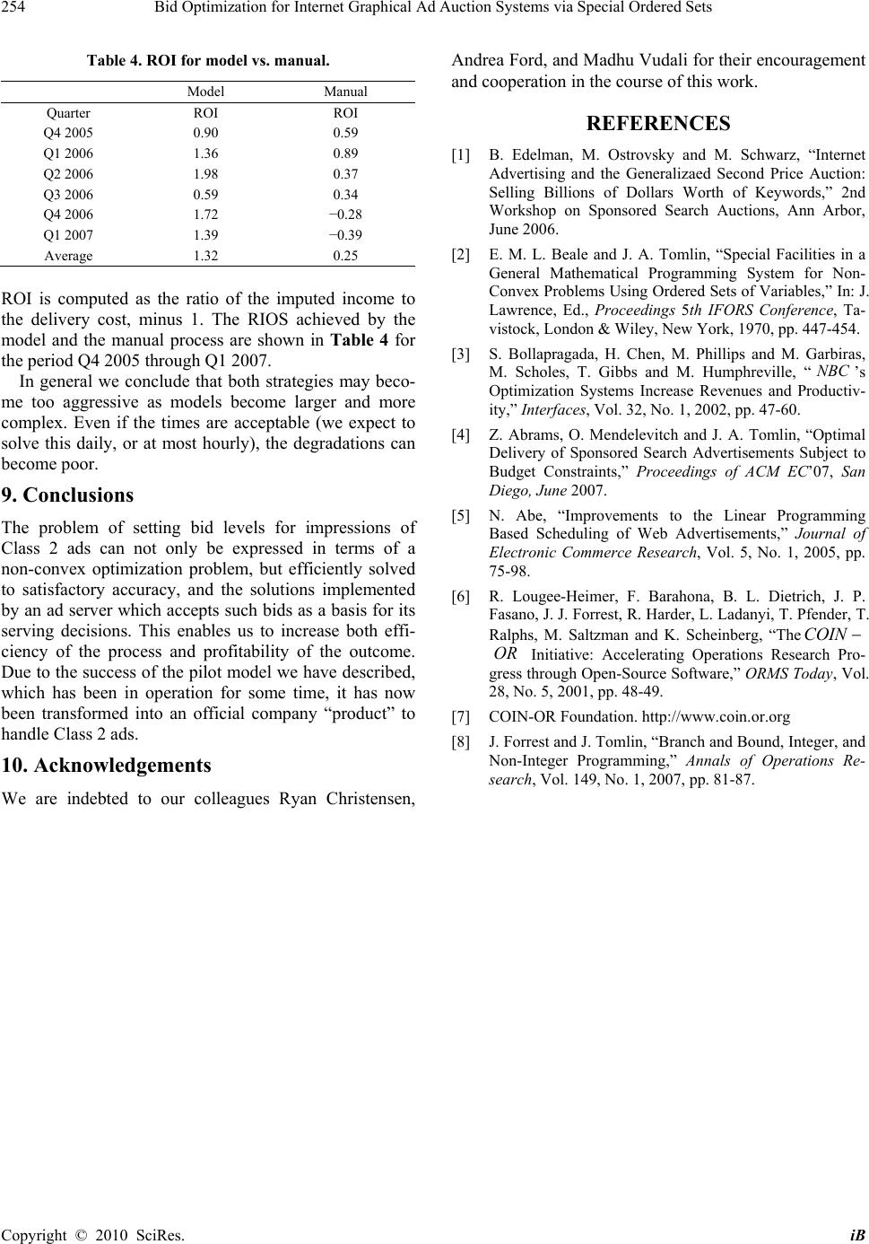

Bid Optimization for Internet Graphical Ad Auction Systems via Special Ordered Sets
254
Table 4. ROI for model vs. manual.
Model Manual
Quarter ROI ROI
Q4 2005 0.90 0.59
Q1 2006 1.36 0.89
Q2 2006 1.98 0.37
Q3 2006 0.59 0.34
Q4 2006 1.72 −0.28
Q1 2007 1.39 −0.39
Average 1.32 0.25
ROI is computed as the ratio of the imputed income to
the delivery cost, minus 1. The RIOS achieved by the
model and the manual process are shown in Table 4 for
the period Q4 2005 through Q1 2007.
In general we conclude that both strategies may beco-
me too aggressive as models become larger and more
complex. Even if the times are acceptable (we expect to
solve this daily, or at most hourly), the degradations can
become poor.
9. Conclusions
The problem of setting bid levels for impressions of
Class 2 ads can not only be expressed in terms of a
non-convex optimization problem, but efficiently solved
to satisfactory accuracy, and the solutions implemented
by an ad server which accepts such bids as a basis for its
serving decisions. This enables us to increase both effi-
ciency of the process and profitability of the outcome.
Due to the success of the pilot model we have described,
which has been in operation for some time, it has now
been transformed into an official company “product” to
handle Class 2 ads.
10. Acknowledgements
We are indebted to our colleagues Ryan Christensen,
Andrea Ford, and Madhu Vudali for their encouragement
and cooperation in the course of this work.
REFERENCES
[1] B. Edelman, M. Ostrovsky and M. Schwarz, “Internet
Advertising and the Generalizaed Second Price Auction:
Selling Billions of Dollars Worth of Keywords,” 2nd
Workshop on Sponsored Search Auctions, Ann Arbor,
June 2006.
[2] E. M. L. Beale and J. A. Tomlin, “Special Facilities in a
General Mathematical Programming System for Non-
Convex Problems Using Ordered Sets of Variables,” In: J.
Lawrence, Ed., Proceedings 5th IFORS Conference, Ta-
vistock, London & Wiley, New York, 1970, pp. 447-454.
[3] S. Bollapragada, H. Chen, M. Phillips and M. Garbiras,
M. Scholes, T. Gibbs and M. Humphreville, “NB
C
’s
Optimization Systems Increase Revenues and Productiv-
ity,” Interfaces, Vol. 32, No. 1, 2002, pp. 47-60.
[4] Z. Abrams, O. Mendelevitch and J. A. Tomlin, “Optimal
Delivery of Sponsored Search Advertisements Subject to
Budget Constraints,” Proceedings of ACM EC’07, San
Diego, June 2007.
[5] N. Abe, “Improvements to the Linear Programming
Based Scheduling of Web Advertisements,” Journal of
Electronic Commerce Research, Vol. 5, No. 1, 2005, pp.
75-98.
[6] R. Lougee-Heimer, F. Barahona, B. L. Dietrich, J. P.
Fasano, J. J. Forrest, R. Harder, L. Ladanyi, T. Pfender, T.
Ralphs, M. Saltzman and K. Scheinberg, “TheCOIN

OR Initiative: Accelerating Operations Research Pro-
gress through Open-Source Software,” ORMS Today, Vol.
28, No. 5, 2001, pp. 48-49.
[7] COIN-OR Foundation. http://www.coin.or.org
[8] J. Forrest and J. Tomlin, “Branch and Bound, Integer, and
Non-Integer Programming,” Annals of Operations Re-
search, Vol. 149, No. 1, 2007, pp. 81-87.