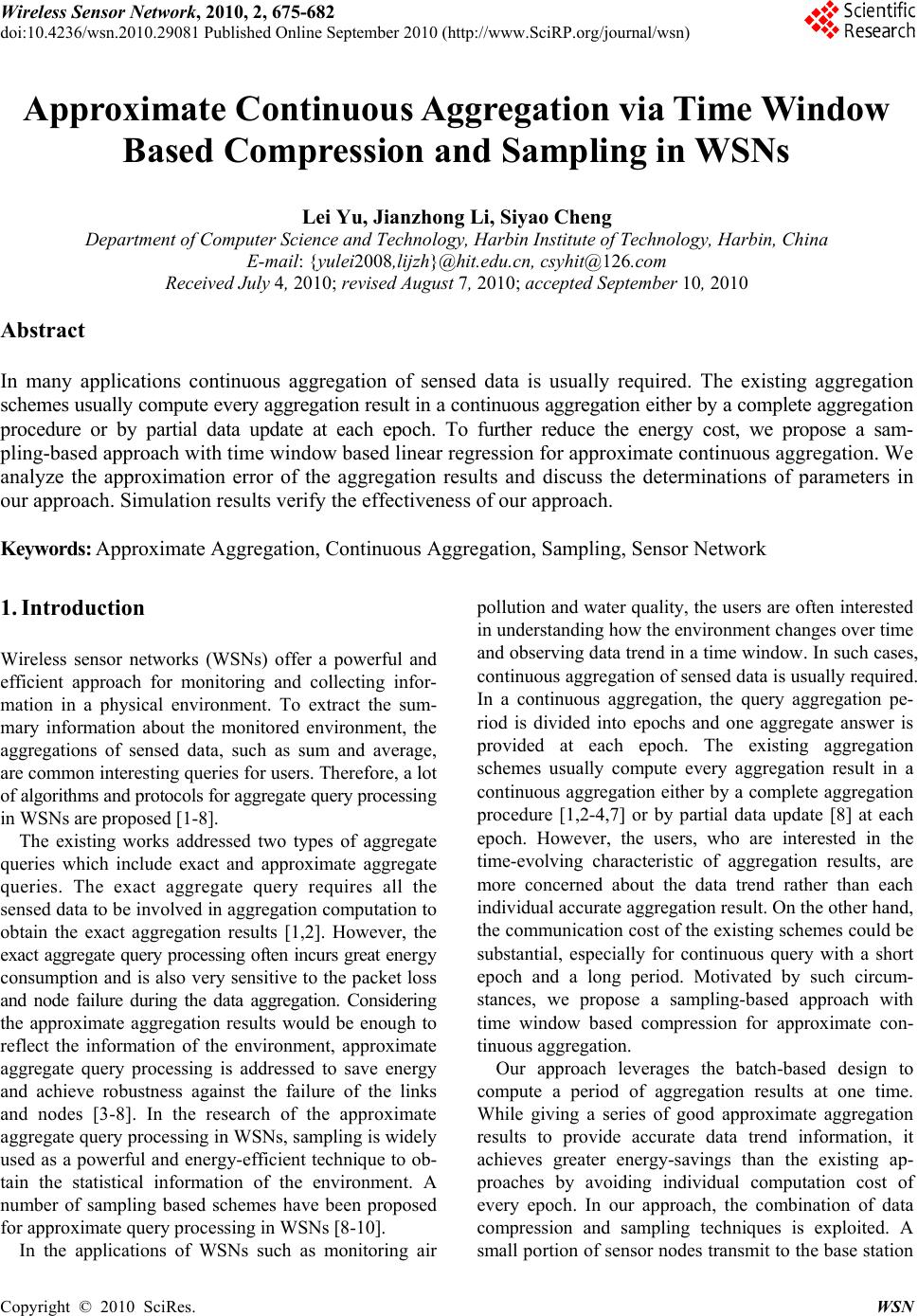Wireless Sensor Network, 2010, 2, 675-682
doi:10.4236/wsn.2010.29081 Published Online September 2010 (http://www.SciRP.org/journal/wsn)
Approximate Continuous Aggregation via Time Window
Based Compression and Sampling in WSNs
Lei Yu, Jianzhong Li, Siyao Cheng
Department of Computer Science and Technology, Harbin Institute of Technology, Harbin, China
Received July 4, 2010; revised August 7, 2010; accepted September 10, 2010
Abstract
In many applications continuous aggregation of sensed data is usually required. The existing aggregation
schemes us ually comput e every aggrega tion resu lt in a con tinuous a ggregat ion eith er by a co mplete aggr egat i o n
procedure or by partial data update at each epoch. To further reduce the energy cost, we propose a sam-
pling-based approach with time window based linear regression for approximate continuous aggregation. We
analyze the approximation error of the aggregation results and discuss the determinations of parameters in
our approach. Simulation results verify the effectiveness of our approach.
Keywords: Approximate Aggregation, Continuous Aggregation, Sampling, Sensor Network
1. Introduction
Wireless sensor networks (WSNs) offer a powerful and
efficient approach for monitoring and collecting infor-
mation in a physical environment. To extract the sum-
mary information about the monitored environment, the
aggregations of sensed data, such as sum and average,
are common interesting queries for users. Therefore, a lot
of algorithms and protocols for aggregate query processin g
in WSNs are proposed [1-8].
The existing works addressed two types of aggregate
queries which include exact and approximate aggregate
queries. The exact aggregate query requires all the
sensed data to be involved in aggregation computation to
obtain the exact aggregation results [1,2]. However, the
exact aggregate query processing often incurs great energy
consumption and is also very sensitive to the packet loss
and node failure during the data aggregation. Considering
the approximate aggregation results would be enough to
reflect the information of the environment, approximate
aggregate query processing is addressed to save energy
and achieve robustness against the failure of the links
and nodes [3-8]. In the research of the approximate
aggregate query processing in WSNs, sampling is widely
used as a powerful and energy-efficient technique to ob-
tain the statistical information of the environment. A
number of sampling based schemes have been proposed
for approximate query processing in WSNs [8-10].
In the applications of WSNs such as monitoring air
pollution and water quality, the users are often interested
in understanding how the environment changes over time
and observing da ta trend in a time window. In such cases,
continuous aggr egation of sensed data is usually req uired.
In a continuous aggregation, the query aggregation pe-
riod is divided into epochs and one aggregate answer is
provided at each epoch. The existing aggregation
schemes usually compute every aggregation result in a
continuous aggregation either by a complete aggregation
procedure [1,2-4,7] or by partial data update [8] at each
epoch. However, the users, who are interested in the
time-evolving characteristic of aggregation results, are
more concerned about the data trend rather than each
individual accurate aggregation result. On the other hand,
the communication cost of the existing schemes could be
substantial, especially for continuous query with a short
epoch and a long period. Motivated by such circum-
stances, we propose a sampling-based approach with
time window based compression for approximate con-
tinuous aggregation.
Our approach leverages the batch-based design to
compute a period of aggregation results at one time.
While giving a series of good approximate aggregation
results to provide accurate data trend information, it
achieves greater energy-savings than the existing ap-
proaches by avoiding individual computation cost of
every epoch. In our approach, the combination of data
compression and sampling techniques is exploited. A
small portion of sensor nodes transmit to the base station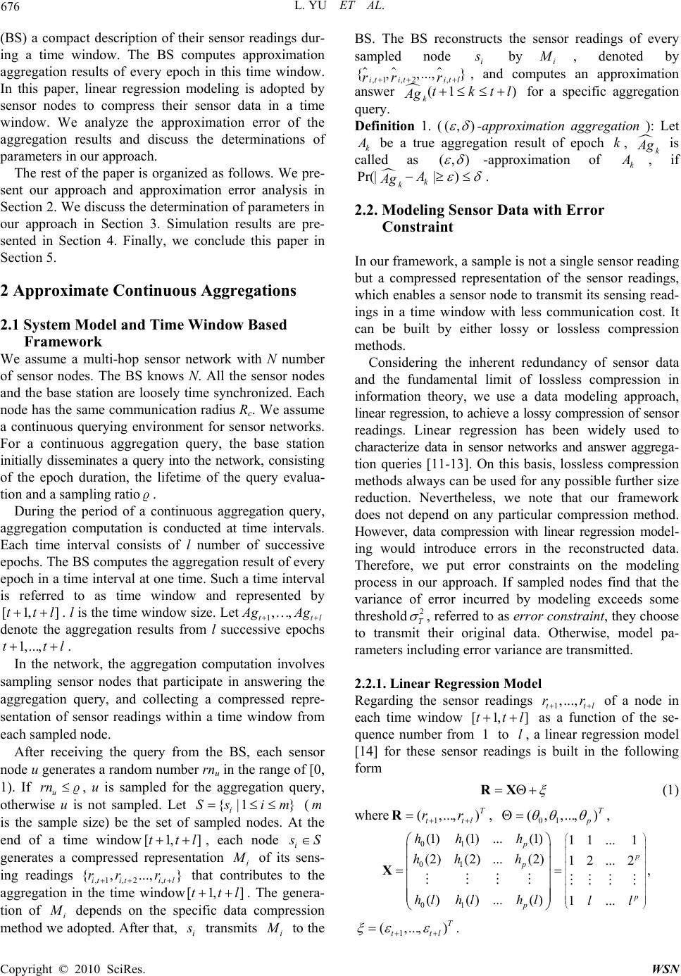

L. YU ET AL.
676
(BS) a compact description of their sensor readings dur-
ing a time window. The BS computes approximation
aggregation results of every epoch in this time window.
In this paper, linear regression modeling is adopted by
sensor nodes to compress their sensor data in a time
window. We analyze the approximation error of the
aggregation results and discuss the determinations of
parameters in our approach.
The rest of the paper is organized as follows. We pre-
sent our approach and approximation error analysis in
Section 2. We discuss the determination of parameters in
our approach in Section 3. Simulation results are pre-
sented in Section 4. Finally, we conclude this paper in
Section 5.
2 Approximate Continuous Aggregations
2.1 System Model and Time Window Based
Framework
We assume a multi-hop sensor network with N number
of sensor nodes. The BS knows N. All the sensor nodes
and the base station are loosely time synchronized. Each
node has the same communication radius Rc. We assume
a continuous querying environment for sensor networks.
For a continuous aggregation query, the base station
initially disseminates a query into the network, consisting
of the epoch duration, the lifetime of the query evalua-
tion and a sampling ratio.
During the period of a continuous aggregation query,
aggregation computation is conducted at time intervals.
Each time interval consists of l number of successive
epochs. The BS computes the aggregation result of every
epoch in a time interval at one time. Such a time interval
is referred to as time window and represented by
[1 ]ttl . l is th e time window size. Let1…
ttl
A
gAg



denote the aggregation results from l successive epochs
1,...ttl
.
In the network, the aggregation computation involves
sampling sensor nodes that participate in answering the
aggregation query, and collecting a compressed repre-
sentation of sensor readings within a time window from
each sampled node.
After receiving the query from the BS, each sensor
node u generates a random number rnu in the range of [0,
1). If u rn , u is sampled for the aggregation query,
otherwise u is not sampled. Let {1 }
i
Ss im (m
is the sample size) be the set of sampled nodes. At the
end of a time window[1 ]ttl , each node i
s
S

generates a compressed representation i
M
of its sens-
ing readings 12 {}
ititit l
rr r
 
 that contributes to the
aggregation in the time window[1 ]ttl . The genera-
tion of i
M
depends on the specific data compression
method we adopted. After that, i
s
transmits i
M
to the
BS. The BS reconstructs the sensor readings of every
sampled node i
s
byi
M
, denoted by
12
{,}
ititit l
rr r

 
 
 , and computes an approximation
answer

(1 )
ktktl
Ag

 for a specific aggregation
query.
Definition 1. (()



-approximation aggregation ): Let
k
A
be a true aggregation result of epoch k,

k
A
g is
called as ()



-approximation of k
A
, if

Pr( )
k
kA
Ag



.
2.2. Modeling Sensor Data with Error
Constraint
In our framework, a sample is not a single sensor reading
but a compressed representation of the sensor readings,
which enables a sensor node to transmit its sensing read-
ings in a time window with less communication cost. It
can be built by either lossy or lossless compression
methods.
Considering the inherent redundancy of sensor data
and the fundamental limit of lossless compression in
information theory, we use a data modeling approach,
linear regression, to achieve a lossy compression of senso r
readings. Linear regression has been widely used to
characterize data in sensor networks and answer aggrega-
tion queries [11-13]. On this basis, lossless compression
methods always can be used for any possible further size
reduction. Nevertheless, we note that our framework
does not depend on any particular compression method.
However, data compression with linear regression model-
ing would introduce errors in the reconstructed data.
Therefore, we put error constraints on the modeling
process in our approach. If sampled nodes find that the
variance of error incurred by modeling exceeds some
threshold 2
T

, referred to as error constraint, they choose
to transmit their original data. Otherwise, model pa-
rameters including error variance are transmitted.
2.2.1. Linear Regression Model
Regarding the sensor readings 1ttl rr

 of a node in
each time window [1 ]ttl

 as a function of the se-
quence number from 1 to l, a linear regression model
[14] for these sensor readings is built in the following
form


RX (1)
where 1
(...)
T
ttl
rr

R, 01 (... )T
p
   ,
01
01
01
(1)(1) ...(1)11...1
(2)(2) ...(2)1 2 ... 2
()() ...()1...
p
p
p
p
p
hh h
hh h
hl hlhlll




















X  
1
( ... )T
ttl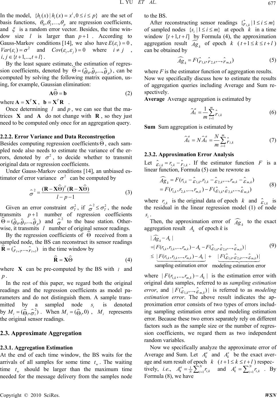
 

 .

L. YU ET AL.
677
In the model, {() ()0}
i
ii
hx hxxip
are the set of
basis functions, 01 …
p

  are regression coefficients,
and

is a random error vector. Besides, the time win-
dow size l is larger than1p. According to
Gauss-Markov conditions [14], we also have() 0
i
E


,
2
()
i
Var

  and ()0
ij
Cov

  where ij

,
{1... }ijttl .
By the least square estimate, the estimation of regres-
sion coefficients, denoted by

 
01
(...)
p



 , can be
computed by solving the following matrix equation, us-
ing, for example, Gaussian elimination:

Ab (2)
where T
AXX
, T bXR .
Once determining l andp, we can see that the ma-
trices X and A do not change with R, so they just
need to be computed only once for an aggregation query.
2.2.2. Error Variance and Dat a Rec ons tru ction
Besides computing regression coefficients

, each sam-
pled node also needs to estimate the variance of the er-
rors, denoted by 2

, to decide whether to transmit
original data or regression coefficients.
Under Gauss-Markov conditions [14], an unbiased es-
timator of error variance 2

can be computed by



2()()
1
T
lp

 

RXRX (3)
Given an error constraint 2
T

, if

22
T


, the node
transmits 1p number of regression coefficients

 
01
(...)
p


  and

2

to the base station. Other-
wise, it transmits l number of original sensor readings.
By the regression coefficients of

 received from a
sampled node, the BS can reconstruct its sensor readings

1
( ... )
ttl
rr

R in the time window by


RX (4)
where X can be pre-computed by the BS with l and
p.
In the rest of this paper, we regard both the original
readings and the regression coefficients as model pa-
rameters and do not distinguish them. A sample trans-
mitted by a sampled node i
s
is denoted
by
 
2
()
iii
M


. When

(0)
ii
M


, i
M
represents
the original sensor readings.
2.3. Approximate Aggregation
2.3.1. Aggre ga tion Estimation
At the end of each time window, the BS waits for the
arrivals of all samples for some time w t. The waiting
time w
t should be larger than the maximum time
needed for the message delivery from the samples node
to the BS.
After reconstructing sensor readings {1 }
ik im
r

of sampled nodes {1 }
i
s
im

 at epoch k in a time
window [1 ]ttl

 by Formula (4), the approximation
aggregation result

k
A
g of epoch k (1tktl )
can be obtained by

12
(...)
kk mk
kF
Ag rr r



 (5)
where F is the estimator function of aggregation results.
Now we specifically discuss how to estimate the results
of aggregation queries including Average and Sum re-
spectively.
Average Average aggregation is estimated by

1
1m
a
kik
i
Ar
m

 (6)
Sum Sum aggregation is estimated by

1
m
aa
kk ik
i
N
ANA r
m


 (7)
2.3.2. Approxi m ation Error Analysis
Let

ik ik
ik rr





. If the estimator function
F
is a
linear function, Formula (5) can be rewrote as

 
 
12
12
12 12
(... )
(... ) (...)
kk mk
kk mk
k
kk mkkk mk
Fr rr
Ag
Fr rrF
 
 
 


  

  (8)
where ik
r

is the original data of epoch k and

ik


is
the residual in the linear regression model (1) of node
i
s
.
Then, the approximation error of

k
A
g to the exact
aggregation result k
A
of epoch k is

 
 
12 12
12 12
(...)(...)
(... )(...)
samplingestimation errormodeling estimation error
k
k
kk mkkkk mk
kk mkkkk mk
A
Ag
Fr rrAF
Fr rrAF
 
 
  
  

  

 
 
(9)
where 1
( ...)
kmk k
F
rr A


  is the estimation error with
original data samples, referred to as sampling estimation
error, and

1
( ...)
kmk
F




is referred to as modeling
estimation error. The above result indicates the ap-
proximation error consists of two types of errors includ-
ing sampling estimation error and modeling estimation
error. Because these two errors separately rely on differe nt
factors such as the sample size or the number of regres-
sion coefficients, we regard them as two independent
random variables.
Now we specifically analyze the approximate error of
Average and Sum. Let a
k
A
and
s
k
A
be the exact aver-
age and sum result of epoch k (1tktl ) respec-
tively, i.e., 11
N
a
kik Ni
A
r


 and 1
N
s
kik
i
A
r


. By
Formula (8), we have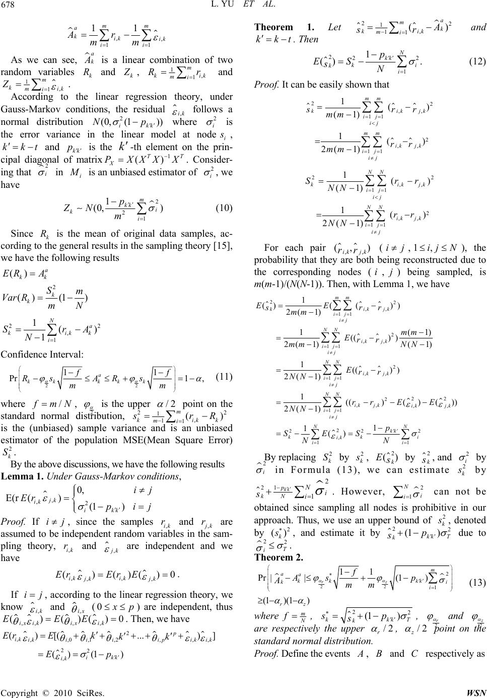

L. YU ET AL.
678


11
11
mm
a
kik ik
ii
Ar
mm





As we can see,

a
k
A
is a linear combination of two
random variables k R and k
Z
, 11
m
kik
mi
Rr


 and

11
m
kik mi
Z



.
According to the linear regression theory, under
Gauss-Markov conditions, the residual

ik

 follows a
normal distribution 2
(0 (1))
ikk
Np 

 where 2
i

is
the error variance in the linear model at nodei
s
,
kkt
 and kk p is the k

-th element on the prin-
cipal diagonal of matrix1
()
TT
X
PXXXX

. Consider-
ing that

2
i

in i
M
is an unbiased esti mator of 2
i

, we
have

2
21
1
(0 )
m
kk i
ki
p
ZN m





 (10)
Since k
R is the mean of original data samples, ac-
cording to the general results in the sampling theory [15],
we have the following results
() a
kk
ER A
2
()(1)
k
k
Sm
Var RmN

22
1
1()
1
Na
kikk
i
SrA
N



Confidence Interval:
22
11
Pr 1
a
kk kkk
ff
Rs ARs
mm










 
(11)
where
f
mN, 2


is the upper 2

 point on the
standard normal distribution, 22
111()
m
kikk
mi
srR




is the (unbiased) sample variance and is an unbiased
estimator of the population MSE(Mean Square Error)
2
k
S.
By the above discussions, we have the following results
Lemma 1. Under Gauss-Markov conditions,
E(r

,
,2
0,
()(1)
jk
ik
ikk
ij
Er pij 







Proof. If ij, since the samples ik r and
j
k
r

are
assumed to be independent random variables in the sam-
pling theory, ik r and

j
k

 are independent and we
have

()()()0
ik ik jk jk
ErEr E

 

.
If ij, according to the linear regression theory, we
know

ik

 and

ix

 (0
x
p) are independent, thus




()()()0
ix ikixik
EEE
 
 
 . Then, we have








2
01 2
22
()[(... )]
() (1)
p
ik ikiiiipik ik
ikk ik
ErEk kk
Ep

 


 






Theorem 1. Let

22
111()
a
mk
ik
kmiA
sr



 and
kkt


. Then
222
1
1
() N
kk
ki
ki
p
ES
sN







 (12)
Proof. It can be easily shown that
22
11
2
11
1()
(1)
1()
2( 1)
mm
ik jk kij
ij
mm
ik jk
ij
ij
srr
mm
rr
mm














22
11
2
11
1()
(1)
1()
2( 1)
NN
kikjk
ij
ij
NN
ik jk
ij
ij
Srr
NN
rr
NN












For each pair ()
ik jk
rr



 (ij,1ij N ), the
probability that they are both being reconstructed due to
the corresponding nodes (i,j) being sampled, is
m(m-1)/(N(N-1)). Then, with Lemma 1, we have

22
11
2
11
2
11
22 2
11
2
1
1
()( ())
2( 1)
1(1)
(())
2( 1)(1)
1(())
2( 1)
1(()( )())
2( 1)
1
mm
ik jk
kij
ij
NN
ik jk
ij
ij
NN
ik jk
ij
ij
NN
ik jkik jk
ij
ij
ki
EE
srr
mm
mm
Err
mm NN
Err
NN
rr EE
NN
SN










 





















222
1
1
()
NN
kk
ki ik i
p
ES
N







By replacing 2
k
S by 2
k
s
, 2 ()
k
E
s
 by 2
k
s
, and 2
i

by

2
i

in Formula (13), we can estimate 2
k
s
by
 1 22
1
kk
p
kN
Ni
i
s





. However, 
2
1
N
i
i


 can not be
obtained since sampling all nodes is prohibitive in our
approach. Thus, we use an upper bound of 2
k
s
, denoted
by 2
()
k
s
, and estimate it by 22
(1 )
kk T kp
s



 due to

22
T i


.
Theorem 2.


22
2
1
11
Pr(1 )
(1 )(1 )
rz
m
aa
kk kk
ki
i
rz
f
As p
Amm




 
 

 

 
 

 

 
 
 (13)
where m
N
f

, 22 (1 )
kkkT k
sp
s



, 2
r


and 2
z


are respectively the upper 2
r

, 2
z

 point on the
standard normal distribution.
Proof. Define the events
A
, B and C respectively as

L. YU ET AL.
679



22
2
2
2
1
2
1
11
1
1(1 )
rz
r
z
m
aa
kkk i
i
a
kk
k
m
kkk i
i
f
AAA smm
f
BRAs m
CZ p
m













  

 
 


Because 22
k
k
s
s, by Formula (12) we have
2
1
Pr()Pr()1
r
f
a
kk kr
m
BRAs




 
Since

2
2
1
1
(0)
kk m
pi
kmi
ZN




 ,

2
2
1
1
Pr(1 )1
z
m
i
kkkz
i
Zp
m













By Formula (9), we have

aaa
kkkk k
A
ARA Z
.
When inequalities B and C are satisfied,
A
must
hold. Because sampling and modeling errors are inde-
pendent random variables, so B and C are inde-
pendent events. Then, we have
Pr()Pr()Pr( )Pr( )(1)(1)
rz
ABCBC

  
Let

22
2
1
11
(1 )
rz
m
kk kk i
i
f
sp
mm

 





.
Since


sa
kk
kk
NNRNZ
AA
, we can easily derive the
following results from the above analysis of average:

Pr(1 )(1)
ss
kk rz kAN A





 (14)
Here Formulas (13) and (14) give the approximation
error k

(k N

) of Average (Sum) aggregation with the
probability guarantee (1)(1)
rz

 .
3. Parameter Determination
From Formulas (13) and (14) we can see that with given
the probability guarantee, i.e., r

and
z

, the approxi-
mation error depends on the error constraint 2
T

and the
sample size m. In this section we discuss the selection
of their values with the desired error bound for k

by
users, denoted byT

.
3.1. Error Constraint 2
T

As shown in Formula (3),

i

indicates the average er-
ror for the data reconstructed in a time window. Thus,
T

specifies the maximum degree of the average error
that the user can tolerate for the reconstructed data. A
larger T

would allow larger errors in the reconstructed
data and may enlarge the approximation error. On the
other hand, a larger T

gives the sampled nodes more
chances to transmit their model parameters instead of
their original data and further reduce the communication
cost. Thus, the trade-off exists between communication
cost and approximation error.
Here we provide one possible solution to determ ine2
T

.
During the first time window of aggregation, all sampled
nodes transmit their original data to the BS. The BS fits
the specified model to these data and computes the mod-
eling errors 2
ˆ
{|1}
iim
  for all sampled nodes. A
histogram is computed to count the number of error val-
ues falling into each bin, which reflects the quality of
data modeling for the sensor network. According to this
frequency distribution, the user can select a value of 2
T

as large as possible while ensuring an acceptable ap-
proximation error. Finally, the BS broadcasts 2
T

to the
sensor network and each sensor node works on the new
error variance constraint. This procedure could be con-
ducted reactively when substantial sampled nodes start to
continuously transmit their original data, which indicates
the changes of the nature of data in the sensor network.
In our experiments on real data set, we show linear re-
gression well characterizes the sensor data and incur few
original data transmissions even with a small error vari-
ance constrain.
3.2. Sampling Ratio 
From Formulas (13) and (14), a larger sample size m
enables a smaller approximation error.
It is easily shown that we can relax k

to
22
11
rz
f
kk T
mm
s






without changing the inequality relationship with the
probability guarantee(1 )(1 )
rz



 in Formulas (13)
and (14). We consider the least sample size to satisfy
kT



for any k in[1 ]ttl

 . With an approxima-
tion of /0fmN

 (for relative small sample size
and large population), we have
22
11
rz
kTT
mm
s


 



which should hold for any k in [1 ]ttl . Then, we
can obtain the least sample size k m required by epoch k
in the time window [1 ]ttl

 to ensure k

is less
than a threshold T

22
2
(), 1
rz
kT
kT
s
mtktl





  (15)
For each epoch k in [1 ]ttl , if the BS finds
k
mm

, it can issue another sampling request to obtain
k
mm

samples. However, k
s
 cannot be obtained be-
fore sampling, we give the following estimation if the

L. YU ET AL.
680
upper bound rmax and lower bond rmin of sensor readings
are known
*2
max min
1
1()
12
m
ki
rr
sm

 (16)
We can obtain an estimation of the required sample
size, denoted by mr, for all epochs in the time window
[1 ]ttl by inserting Formula (15) into Formula (16).
The sampling ratio  is set to be not less than mr/N.
3.3. Time Window Size l
When all sampled nodes transmit their original data, the
approximation error includes only the sampling estima-
tion error and no modeling estimation error. Thus, the
aggregation computation with original data needs a less
sample size than with the compressed data by modeling
to achieve the same approximation erro r. Let o m be the
sample size needed to obtain ()
T

 -approximation
aggregation by collecting the original data, then
2
1o
o
f
kT
m
s



 where o m
o
N
f. With the approxima-
tion of /0
oo
fmN,
2
22
()
okT
ms


 
On the other hand, we have
22
1(1 )(1 )r
rz r





 
As above, we also have 22
z




.
According to the above discussion on sampling ratio,
we have
22 22
22
22
2
22 2
22 2
22
22
22
2
()()
() ()
()
()
()
()
(1 )
rzrz kTT kT
t
okT k
kT kT
kk
kT T
k k
ss
m
mss
ss
ss
s
s s
 




 
 




 






(17)
Without data modeling compression, the aggregation
requires (1)
o
ml original data tran smissions for a time
window to achieve the approximation error T

. With
the data modeling compression, our scheme requires
(2)mp data transmissions to achieve the approxima-
tion error T

. To achieve energy savings, we should
have (1)/( 2)1
ot
ml mp, then
2
1( 2)( 2)(1)
tT
ok
m
lp p
ms

  
In the case of Tk S

, 12
T
k
s


, we could set
14( 2)lp .
4. Simulation Evaluation
To measure the performance of our secure aggregation
scheme, we simulate a sensor network based on the data
from a real world deployment with 54 sensor nodes (ID
from 1 -54) in the Intel Research lab, which includes a
trace of sensor readings collected between February and
April,2004 , node location and network connectivity in-
formation. The sensors collected time-stamped humidity,
temperature and voltage values in 31 second intervals.
We use the first 2000 epochs of the data set in the day
03/08 with the largest size among all days and assume a
continuous aggregation query on the temperature attribute
during this period. The periodic aggregation is conducted
on it with a time window size 40l, i.e., 50 time win-
dows. In the linear regression model, we let3p

.
To show the performance of linear regression model
for describing sensor data, we investigate the distribution
of error variance and its impact on data transmission for
all sensor nodes.
Figure 1 shows temperature readings (in degrees Cel-
sius) of 52 sensor nodes in 2000 successive epochs,
which are used for our simulation. Figure 2 shows the
error variance of linear regression model in every time
window for all sensor nodes. For all time windows, all
the sensor nodes have error variances less than 0.2. Fig-
ure 3 shows under different choice of error constraint
2
T

, the number of sensor nodes which has a larger mod-
eling error variance than 2
T

in each time window. We
can conclude most of sensor nodes at most of time win-
dows are consistent with variance constraint.
When 2007
T
  , less than 10% of sensor nodes ex-
ceed 2
T

; when 201
T
  , the number decreases to
2%.Our experiment indicates only a small portion of
sampled node will transmit their original data.
Figure 1. Temperature readings (in degrees Celsius) of 52
sensor nodes in 2000 successive epochs (excluding two
nodes with incomplete data and one node with abnormal
data).

L. YU ET AL.
681
Figure 2. The error variances of linear regression model in
all sensor nodes for each time window.
Figure 3. the number of sensor nodes with error variance
2
T

 in each time window.
Assuming = 0.4 and 202
T


, Figure 4 shows the
difference between the average aggregation result esti-
mated by sampling with time window based compression
and the aggregation result estimated by sampling with
original data transmission in every epoch. As we can see,
the difference is in [-0.2, 0.25]. It indicates that our
approach with data compression can obtain the estima-
tion of average aggregations close to those obtained by
the approach without data compression, even when the
sample size is the same. It also indicates our approach
achieves the energy efficiency while obtaining the ap-
proximate estimations, since in each time window only
five numbers are sent from each sampled node.
Figure 4. The difference between two average aggregation
results respectively estimated by the approaches with and
without data compression in every epoch.
5. Conclusions
In this paper we propose a sampling-based approach with
time window based linear regression for approximate
continuous aggregation. The approximation error of the
aggregation results is analyzed. The determination of
parameters in our approach is also discussed. By simula-
tion results on real data set we verify th e effectiveness of
our approach.
5. References
[1] S. Madden, M. J. Franklin, J. M. Hellerstein and W.
Hong, “The Design of an Acquisitional Query Processor
for Sensor Networks,” Proceedings of International
Conference on Management on Data, California, 2003,
pp. 491-502.
[2] S. Madden, M. J. Franklin, J. M. Hellerstein and W.
Hong, “TAG: A Tiny Aggregation Service for Ad Hoc
Sensor Networks,” Proceedings of the 5th Symposium on
Operating Systems Design and Implementation, New
York, 2002, pp. 131-146.
[3] J. Considine, F. Li, G. Kollios and J. Byers, “Approxi-
mate Aggregation Techniques for Sensor Databases,” In-
ternational Conference on Data Engineering, Boston,
2004, pp. 449-460.
[4] S. Nath, P. B. Gibbons, S. Seshan and Z. R. Anderson,
“Synopsis Diffusion for Robust Aggregation in Sensor
Networks,” Sensys, 2004, pp. 250-262.
[5] G. Cormode, M. N. Garofalakis, S. Muthukrishnan and R.
Rastogi, “Holistic Aggregates in a Networked World:
Distributed Tracking of Approximate Quantiles,” Pro-
ceedings of International Conference on Management on
Data, 2005, pp. 25-36.
[6] A. Deligiannakis, Y. Kotidis and N. Rossopoulos, “Proc-
essing Approximate Aggregation Queries in Wireless
Senor Networks,” Information Systems, Vol. 31, No. 8,
2006, pp. 770-792.
[7] A. Manjhi, S. Nath and P. B. Gibbons, “Tributaries and
Deltas: Efficient and Robust Aggregation in Sensor Net-
work Streams,” ACM SIGMOD, ACM Press, 2005, pp.
287-298.
[8] S. Y. Cheng, J. Z. LI, Q. Q. Ren and L. Yu, “Bernoulli
Sampling Based (epsilon, delta)-Approximate Aggrega-
tion in Larger-Scale Sensor Networks,” IEEE Interna-
tional Conference on Computer Communications, Cali-
fornia, 2010, pp. 1181-1189.
[9] S. Lin, B. Arai, D. Gunopulos and G. Das, “Region Sam-
pling: Continuous Adaptive Sampling on Sensor Net-
works,” IEEE International Conference on Data Engi-
neering, Cancun, 2008, pp. 794-803.
[10] B. Bash, J. Byers and J. Considine, “Approximately Uni-

L. YU ET AL.
682
form Random Sampling in Sensor Networks,” Proceed-
ings of 1st Workshop on Data Management in Sensor
Networks, August, 2004.
[11] C. Guestrin, P. Bodik, R. Thibaux, M. Paskin and S.
Madden, “Distributed Regression: An Efficient Frame-
work for Modeling Sensor Network Data,” ACM/IEEE
IPSN, 2004, pp. 1-10.
[12] W. Xue, Q. Luo, L. Chen and Y. Liu, “Contour Map
Matching for Event Detection in Sensor Networks,”
SIGMOD, New York, 2006, pp. 145-156.
[13] H. Gupta, V. Navda, S. R. Das and V. Chowdhary, “Effi-
cient Gathering of Correlated Data in Sensor Networks,”
MobiHoc, New York, 2005, pp. 402-413.
[14] A. Sen and M. Srivastava, “Regression Analysis: Theory,
Methods, and Applications,” Springer-Verlag, New York,
1990.
[15] Z. Govindarajulu, “Elements of Sampling Theory and
Methods,” Prentice Hall, New Jersey, 1999.