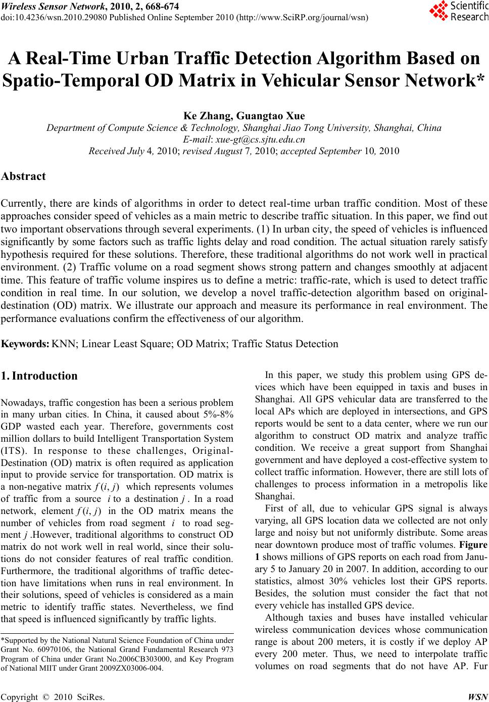Wireless Sensor Network, 2010, 2, 668-674
doi:10.4236/wsn.2010.29080 Published Online September 2010 (http://www.SciRP.org/journal/wsn)
A Real-Time Urban Traffic Detection Algorithm Based on
Spatio-Temporal OD Matrix in Vehicular Sensor Network*
Ke Zhang, Guangtao Xue
Department of C omput e Science & Technolo gy, S han gh ai Ji ao To n g Uni v ersi t y , Shan gh ai, C hi n a
Received July 4, 2010; revised August 7, 2010; accepted September 10, 2010
Abstract
Currently, there are kinds of algorithms in order to detect real-time urban traffic condition. Most of these
approaches consider speed of vehicles as a main metric to describe traffic situation. In this paper, we find out
two important observations through several experiments. (1) In urban city, the speed of vehicles is influenced
significantly by some factors such as traffic lights delay and road condition. The actual situation rarely satisfy
hypothesis required for these solutions. Therefore, these traditional algorithms do not work well in practical
environment. (2) Traffic volume on a road segment shows strong pattern and changes smoothly at adjacent
time. This feature of traffic volume inspires us to define a metric: traffic-rate, which is used to detect traffic
condition in real time. In our solution, we develop a novel traffic-detection algorithm based on original-
destination (OD) matrix. We illustrate our approach and measure its performance in real environment. The
performance evaluations confirm the effectiveness of our algorithm.
Keywords: KNN; Linear Least Square; OD Matrix; Traffic Status Detection
1. Introduction
Nowadays, traffic congestion has been a serious problem
in many urban cities. In China, it caused about 5%-8%
GDP wasted each year. Therefore, governments cost
million dollars to build Intelligen t Transportation System
(ITS). In response to these challenges, Original-
Destination (OD) matrix is often required as application
input to provide service for transportation. OD matrix is
a non-negative matrix(, )
f
ij which represents volumes
of traffic from a source ito a destinationj. In a road
network, element(,)
f
ij in the OD matrix means the
number of vehicles from road segment i to road seg-
ment j.However, traditional algorithms to construct OD
matrix do not work well in real world, since their solu-
tions do not consider features of real traffic condition.
Furthermore, the traditional algorithms of traffic detec-
tion have limitations when runs in real environment. In
their solutions, speed of vehicles is considered as a main
metric to identify traffic states. Nevertheless, we find
that speed is influenced significantly by traffic lights.
In this paper, we study this problem using GPS de-
vices which have been equipped in taxis and buses in
Shanghai. All GPS vehicular data are transferred to the
local APs which are deployed in intersections, and GPS
reports would be sent to a data center, where we run our
algorithm to construct OD matrix and analyze traffic
condition. We receive a great support from Shanghai
government and have deployed a cost-effective system to
collect traffic information. However, there are still lots of
challenges to process information in a metropolis like
Shanghai.
First of all, due to vehicular GPS signal is always
varying, all GPS location data we collected are not only
large and noisy but not uniformly distribute. Some areas
near downtown produce most of traffic volumes. Figure
1 shows millions of GPS reports on each road from Janu-
ary 5 to January 20 in 2007. In addition , according to our
statistics, almost 30% vehicles lost their GPS reports.
Besides, the solution must consider the fact that not
every vehicle has installed GPS device.
Although taxies and buses have installed vehicular
wireless communication devices whose communication
range is about 200 meters, it is costly if we deploy AP
every 200 meter. Thus, we need to interpolate traffic
volumes on road segments that do not have AP. Fur
*Supported by the National Natural Science Foundation of China unde
r
Grant No. 60970106, the National Grand Fundamental Research 973
Program of China under Grant No.2006CB303000, and Key Program
of National MIIT under Grant 2009ZX03006-004.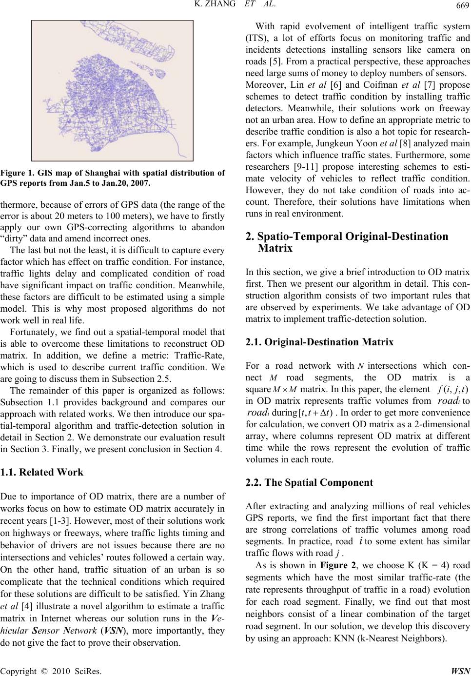

K. ZHANG ET AL.
669
Figure 1. GIS map of Shanghai with spatial distribution of
GPS reports from Jan.5 to Jan.20, 2007.
thermore, because of errors of GPS data (the range of the
error is about 20 meters to 100 meters), we have to firstly
apply our own GPS-correcting algorithms to abandon
“dirty” data and amend incorrect ones.
The last but not the least, it is d ifficult to captu re every
factor which has effect on traffic condition. For instance,
traffic lights delay and complicated condition of road
have significant impact on traffic condition. Meanwhile,
these factors are difficult to be estimated using a simple
model. This is why most proposed algorithms do not
work well in real life.
Fortunately, we find out a spatial-temporal model that
is able to overcome these limitations to reconstruct OD
matrix. In addition, we define a metric: Traffic-Rate,
which is used to describe current traffic condition. We
are going to discuss them in Subsection 2.5.
The remainder of this paper is organized as follows:
Subsection 1.1 provides background and compares our
approach with related work s. We then introduce our spa-
tial-temporal algorithm and traffic-detection solution in
detail in Section 2. We demonstrate our evaluation result
in Section 3. Finally, we present conclusion in Section 4.
1.1. Related Work
Due to importance of OD matrix, there are a number of
works focus on how to estimate OD matrix accurately in
recent years [1-3]. However, most of their solutions work
on highways or freeways, where traffic lights timing and
behavior of drivers are not issues because there are no
intersections and vehicles’ routes fo llowed a certain way.
On the other hand, traffic situation of an urban is so
complicate that the technical conditions which required
for these solutions are difficult to be satisfied. Yin Zhang
et al [4] illustrate a novel algorithm to estimate a traffic
matrix in Internet whereas our solution runs in the Ve-
hicular Sensor Network (VSN), more importantly, they
do not give the fact to prov e their observation.
With rapid evolvement of intelligent traffic system
(ITS), a lot of efforts focus on monitoring traffic and
incidents detections installing sensors like camera on
roads [5]. From a practical perspective, these approaches
need large sums of money to deploy numbers of sensors.
Moreover, Lin et al [6] and Coifman et al [7] propose
schemes to detect traffic condition by installing traffic
detectors. Meanwhile, their solutions work on freeway
not an urban area. How to define an appropriate metric to
describe traffic condition is also a hot topic for research-
ers. For example, Jungkeun Yoon et al [8] analyzed main
factors which influence traffic states. Furthermore, some
researchers [9-11] propose interesting schemes to esti-
mate velocity of vehicles to reflect traffic condition.
However, they do not take condition of roads into ac-
count. Therefore, their solutions have limitations when
runs in real environment.
2. Spatio-Temporal Original-Destination
Matrix
In this section, we give a brief introduction to OD matrix
first. Then we present our algorithm in detail. This con-
struction algorithm consists of two important rules that
are observed by experiments. We take advantage of OD
matrix to implement traffic-detection so lution.
2.1. Original-Destination Matrix
For a road network with
N
intersections which con-
nect
M
road segments, the OD matrix is a
square
M
M

matrix. In this paper, the element (, ,)
f
ijt
in OD matrix represents traffic volumes from iroad to
iroad during[, )tt t

. In order to get more convenience
for calculation, we convert OD matrix as a 2-dimensional
array, where columns represent OD matrix at different
time while the rows represent the evolution of traffic
volumes in each route.
2.2. The Spatial Component
After extracting and analyzing millions of real vehicles
GPS reports, we find the first important fact that there
are strong correlations of traffic volumes among road
segments. In practice, road ito some extent has similar
traffic flows with road
j
.
As is shown in Figure 2, we choose K (K = 4) road
segments which have the most similar traffic-rate (the
rate represents throughput of traffic in a road) evolution
for each road segment. Finally, we find out that most
neighbors consist of a linear combination of the target
road segment. In our solu tion, we develop this discovery
by using an approach: KNN (k-Nearest Neighbors).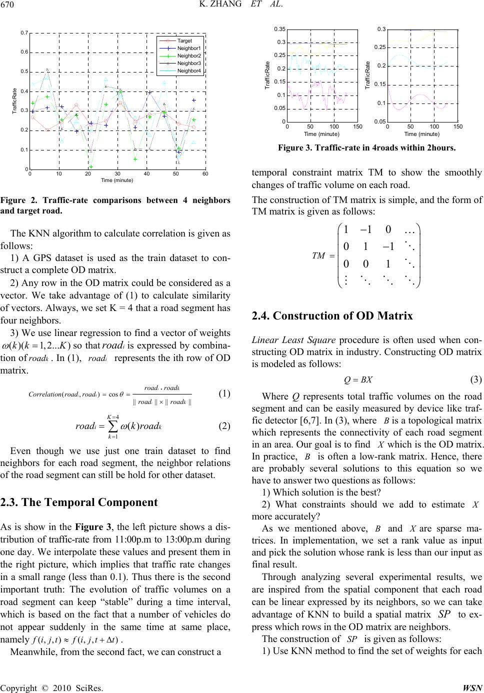

K. ZHANG ET AL.
670
010 2030 40 5060
0
0.1
0.2
0.3
0.4
0.5
0.6
0.7
Time (m i nute)
TrafficRate
Target
Neighbor1
Neighbor2
Neighbor3
Neighbor4
Figure 2. Traffic-rate comparisons between 4 neighbors
and target road.
The KNN algorithm to calculate correlation is given as
follows:
1) A GPS dataset is used as the train dataset to con-
struct a complete OD matrix.
2) Any row in the OD matrix could be considered as a
vector. We take advantage of (1) to calculate similarity
of vectors. Always, we set K = 4 that a road segment has
four neighbors.
3) We use linear regression to find a vector of weights
( )(1,2...)kk K

so thatiroad is expressed by combina-
tion ofkroad . In (1), iroad represents the ith row of OD
matrix.
(, )cos|||| ||||
i
ik
i
k
k
road road
Correlation roadroadroad road 


 (1)
4
1
()
K
ik
k
roadk road 


 (2)
Even though we use just one train dataset to find
neighbors for each road segment, the neighbor relations
of the road segment can still be hold for other dataset.
2.3. The Temporal Component
As is show in the Figure 3, the left picture shows a dis-
tribution of traffic-rate from 11:00p.m to 13:00p.m during
one day. We interpolate these values and present them in
the right picture, which implies that traffic rate changes
in a small range (less than 0.1). Thus there is the second
important truth: The evolution of traffic volumes on a
road segment can keep “stable” during a time interval,
which is based on the fact that a number of vehicles do
not appear suddenly in the same time at same place,
namely (, ,)(, ,)
f
ijtfijt t .
Meanwhile, from the second fact, we can construct a
050100 150
0
0.05
0.1
0.15
0.2
0.25
0.3
0.35
Tim e (m i nut e)
TrafficRate
050100 150
0.05
0.1
0.15
0.2
0.25
0.3
Tim e (minut e)
TrafficRate
Figure 3. Traffic-rate in 4roads within 2hours.
temporal constraint matrix TM to show the smoothly
changes of traffic volume on each road.
The construction of TM matrix is simple, and the form of
TM matrix is given as follows:
110
01 1
00 1
TM 












2.4. Construction of OD Matrix
Linear Least Square procedure is often used when con-
structing OD matrix in industry. Constructin g OD matrix
is modeled as follows:
QBX

(3)
Where Q represents total traffic volumes on the road
segment and can be easily measured by device like traf-
fic detector [6 ,7]. In (3), where
B
is a topological matrix
which represents the connectivity of each road segment
in an area. Our goal is to find Xwhich is the OD matrix.
In practice,
B
is often a low-rank matrix. Hence, there
are probably several solutions to this equation so we
have to answer two questions as follows:
1) Which solution is the best?
2) What constraints should we add to estimate X
more accurately?
As we mentioned above,
B
and Xare sparse ma-
trices. In implementation, we set a rank value as input
and pick the solutio n whose rank is less than our inpu t as
final result.
Through analyzing several experimental results, we
are inspired from the spatial component that each road
can be linear expressed by its neighbors, so we can take
advantage of KNN to build a spatial matrix SP to ex-
press which rows in the OD matrix are neighbors.
The constructio n of SP is given as follows:
1) Use KNN method to find the set of weights for each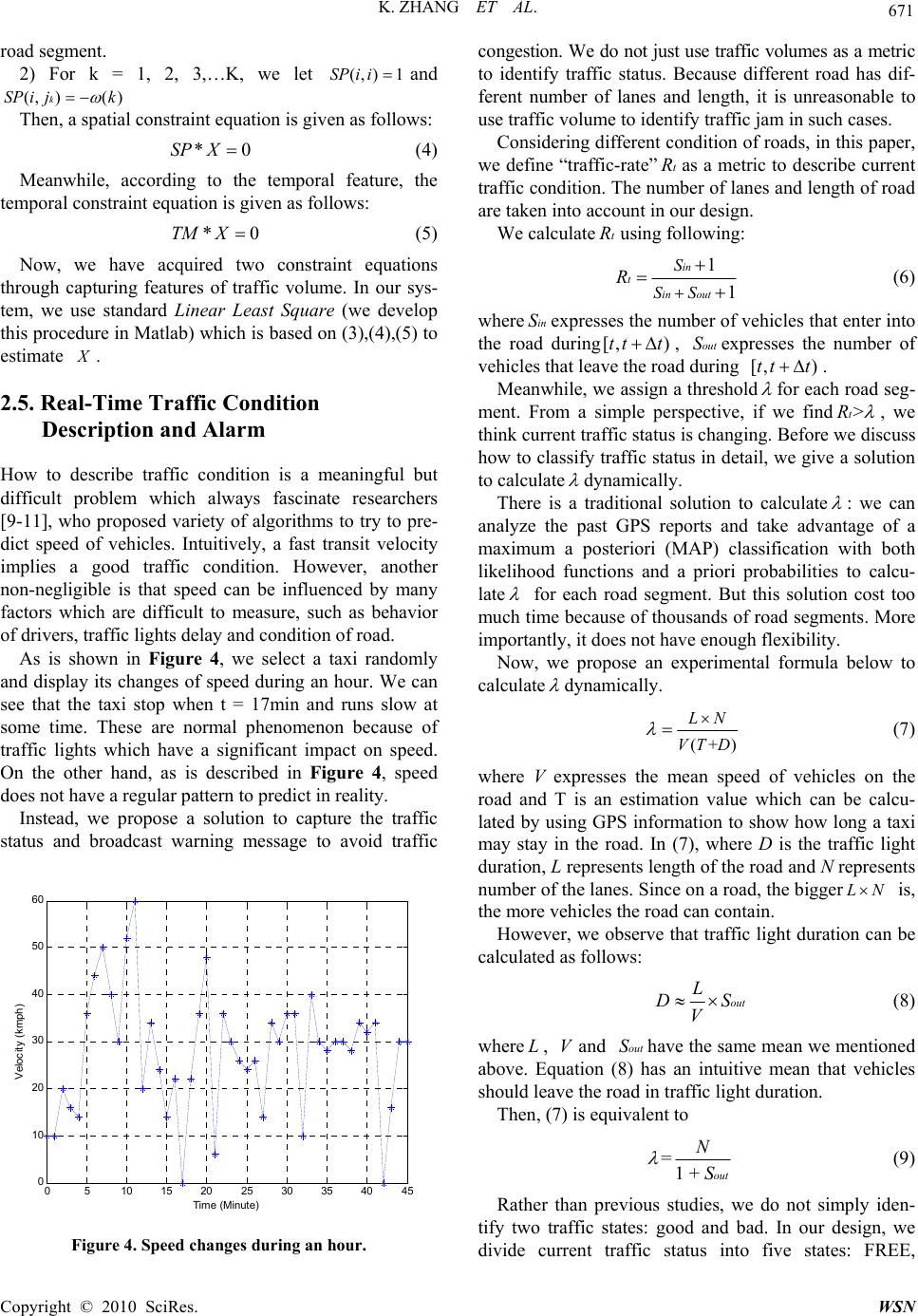

K. ZHANG ET AL.
671
road segment.
2) For k = 1, 2, 3,…K, we let (,) 1SP i i

and
(,)( )kSP ijk


Then, a spatial constraint equation is given as follows:
*0SP X

(4)
Meanwhile, according to the temporal feature, the
temporal constraint equation is given as follows:
*0TM X

(5)
Now, we have acquired two constraint equations
through capturing features of traffic volume. In our sys-
tem, we use standard Linear Least Square (we develop
this procedure in Matlab) which is based on (3),(4),(5) to
estimate
X
.
2.5. Real-Time Traffic Condition
Description and Alarm
How to describe traffic condition is a meaningful but
difficult problem which always fascinate researchers
[9-11], who proposed variety of algorithms to try to pre-
dict speed of vehicles. Intuitively, a fast transit velocity
implies a good traffic condition. However, another
non-negligible is that speed can be influenced by many
factors which are difficult to measure, such as behavior
of drivers, traffic lights delay and conditio n of ro ad.
As is shown in Figure 4, we select a taxi randomly
and display its changes of speed during an hour. We can
see that the taxi stop when t = 17min and runs slow at
some time. These are normal phenomenon because of
traffic lights which have a significant impact on speed.
On the other hand, as is described in Figure 4, speed
does not have a regular pattern to pred ict in reality.
Instead, we propose a solution to capture the traffic
status and broadcast warning message to avoid traffic
05 10 15 20 25 30 35 40 45
0
10
20
30
40
50
60
Tim e (M i nute)
Velocity (kmph)
Figure 4. Speed changes during an hour.
co ngestion. We do not just use traffic volumes as a metri c
to identify traffic status. Because different road has dif-
ferent number of lanes and length, it is unreasonable to
use traffic volume to identify traffic jam in such cases.
Considering different condition of roads, in this p aper,
we define “traffic-rate”tRas a metric to describe current
traffic condition. The number of lan es and length of road
are taken into account in our design.
We calculatetRus ing followi ng:
1
1
in
tin out
S
SS
R

 (6)
where inSexpresses the number of vehicles that enter into
the road during[,)tt t

, outSexpresses the number of
vehicles that leave the road during [,)tt t .
Meanwhile, we assign a threshold

for each road seg-
ment. From a simple perspective, if we find>tR

, we
think current traffic status is changing. Before we discuss
how to classify traffic status in detail, we give a solution
to calculate

dynamically.
There is a traditional solution to calculate

: we can
analyze the past GPS reports and take advantage of a
maximum a posteriori (MAP) classification with both
likelihood functions and a priori probabilities to calcu-
late

for each road segment. But this solution cost too
much time because of thousands of road segments. More
importantly, it does not have enough flexibility.
Now, we propose an experimental formula below to
calculate

dynamically.
(+)
L
N
VT D


 (7)
where V expresses the mean speed of vehicles on the
road and T is an estimation value which can be calcu-
lated by using GPS information to show how long a taxi
may stay in the road. In (7), where D is the traffic light
duration, L represents length of the ro ad an d N represents
number of the lanes. Since on a road, the bigger
L
N

is,
the more vehicles the road can contain.
However, we observe that traffic light duration can be
calculated as follows:
out
L
DS
V
 (8)
whereL, Vand outShave the same mean we mentioned
above. Equation (8) has an intuitive mean that vehicles
should leave the road in traffic light duration.
Then, (7) is equivalent to
=1 + out
N
S
 (9)
Rather than previous studies, we do not simply iden-
tify two traffic states: good and bad. In our design, we
divide current traffic status into five states: FREE,

K. ZHANG ET AL.
672
NORMAL, ALERT, BUSY and OVERLOAD. Since we
must send warning messages of traffic condition to vehi-
cles before traffic condition becomes worse. Another
benefit is that we can make flexible policies when we are
processing traffic information. The rules to identify traf-
fic status on a road are given as follows:
1) 0tR

, the traffic state is FREE;
2) 2tR

  , the traffic state is NORMAL;
3) 23tR

  , the traffic state is ALERT,
4) 34tR

  , the traffic state is BUSY;
5) 41tR

, the traffic state is OVERLOAD.
In our experiments, 0.23

for most cases. When we
detect that current traffic state is ALERT, we start to
send warning message to those related vehicles around
the road.
3. Experiments
3.1. Experimental Setup
We have collected a great number of real traffic data
which are generated in real time by installing GPS de-
vices in taxis and buses from data center in Shanghai.
Even we do not collect all vehicular GPS reports since
some vehicles do not install GPS devices, the evaluations
also show that our solution can work well.
The fields (id, longitude, latitude, velocity, angle,
timestamp) denote the GPS reports, where id identifies a
taxi, the pair (longitude, latitude) shows current coordi-
nates of the taxi, timestamp is the time report, the
pair(velocity, angle) shows current speed and driving
direction of the taxi, which is u sed with Shanghai map to
calculate the short-term destination in our algorithm.
The basic experimental parameters are given as follows:
3.2. Methodology
In order to demonstrate the effectiveness of our solution,
we have developed a mobility model to generate vehicu-
lar GPS reports in a target area. The mobility model con-
sists of three parts:
1) We load GIS map of Shanghai to generate topo-
logical matrix.
2) We set source and destination coordinates for each
node. Traffic light duration is set according to surveys.
3) The nodes send GPS reports randomly and some
nodes do not send. Moreover, for making our simulation
close to real life, we also insert real GPS traces into our
test dataset.
Our initial OD matrix lost elements at some positions
and some elements have error in their value.
At last, we measure performance using the Normal-
ized Mean Absolute Error [4].
,: (,)0
,: (,)0
ˆ
|(,) (,)|
|(,)|
ijMij
ijMij
X
ij Xij
NMAE Xij





 (5)
3.3. Performance
Figure 5 shows the performance of our algorithm ST and
comparison between SRSVD Base [4], KNN, and ST
when GPS reports lost randomly. The default parameters
have been listed in Table 1. We can clearly realize that
ST outperforms the other interpolation algorithms in our
experiment. Sin ce we cap ture s patial and temp oral feat ur es
of traffic flows, ST has more rules and techniques to
interpolate missing values than KNN and SRSVD Base.
Although there is high GPS data loss, ST can still keep a
good performance. From the comparison, we find that
there is significant difference between ST and other
algorithms when GPS-LOSS-PROBABILITY = 0.6.
KNN works well if enough GPS reports have been col-
lected in the datacenter. However, the performance of
KNN decreases sharply when more and more GPS data
lost. Because even we have chosen the best K neighbors
for target route, we still do not have another rule to in-
terpolate traffic flows for target road segment.
SRSVD Base does not work well, since it is to some
extent a pure technique of matrix calculation. Therefore,
it is not able to be adapted to complicated traffic condi-
tion.
3.4. Simulation
The basic experim ental pa ram eters are di splay ed in Tabl e 1.
In followed experiments, we assume that 30% vehicles
do not install GPS devices. Figure 6 shows evolutions of
tR on different road segments. At first, we select three
different road segments randomly in center of Shanghai.
Secondly, we collect the GPS reports on these roads
from 11:00 to 12:00 on Jan.7 2007. At last, we recon-
00.1 0.2 0.3 0.40.5 0.6 0.7 0.80.9
0
0.1
0.2
0.3
0.4
0.5
0.6
0.7
GP S report l oss probability
NM A E
KNN
SRSVD Base
ST
Figure 5. Performance for GPS report loss.

K. ZHANG ET AL.
673
Table 1: Experimental parameters.
Target Area 2
3.5km
Time duration 2hours (11:00-13:00)
Time granularity 5min
Number of road segments 146
Weather Sunny
structed OD matrix using ST to calculatetR. In this
experiment, we find that traffic lights have little effect on
Traffic-Rate and Traffic-Rat e chan ges smoothly.
In order to demonstrate performance of equations of

:
We select 10 road segments randomly and monitor the
traffic volume from 9:00-22:00 on Jan.10 2007. Then we
calculate tRand

every 5 minutes. Meanwhile, we use
mean speed of these vehicles to detect current traffic
status. Finally, we compare our result with pre-defined
traffic state.
Figure 7 shows that the accuracy of our solution and
comparison with traditional policy. Apparently, fro m this
experiment, speed is not a good metric to detect traffic
condition. Since it is often influenced by many factors,
and there are always some vehicles have “strange” driv-
ing behaviors because of habits of drivers. On the other
side, we can clear see that even 90% of accuracy can be
achieved at sometimes. There are also two least values
which are ab out 0.712 at 12:00 and 0.734 at 17:00. Since
they are two important time points when people come off
duty, and traffic condition at that time is difficult to be
captured. But in general, the performance of thresh-
old-based Traffic-Rate is good and adapted to the real
environment.
In Figure 8, the axis of abscissas represents proportion
of vehicles that installed GPS devices. This experiment
010 2030 40 50 60
0
0.1
0.2
0.3
0.4
0.5
0.6
0.7
0.8
Time (Mi nut e)
Traffic-Rate
road1
road2
road3
Figure 6. Traffic-Rate changes during an hour on 3 roads.
0246810 1214 16
0
0.1
0.2
0.3
0.4
0.5
0.6
0.7
0.8
0.9
1
Tim e (Hour)
Accuracy
Traffic-rate
Speed
Figure 7. Accuracy of threshold-based Traffic-Rate and
mean speed of vehicles.
0.5 0.55 0.60.65 0.70.750.8 0.85 0.9 0.951
0
0. 1
0. 2
0. 3
0. 4
0. 5
0. 6
0. 7
0. 8
0. 9
1
Ve hi cles Instal li ng G PS Devices
Accuracy
Accuracy
Figure 8. Accuracy of threshold-based Traffic-Rate.
proves that the more vehicles send GPS reports, the bet-
ter performance of our algorithm is.
4. Conclusions
In this paper, we have presented a practical solution to
detect traffic condition which is based on OD matrix in
an urban city by using a cost-effective system of vehicle
GPS sensors. Our algorithm consists of spatial and tem-
poral components which are based on neighbors of roads
and stability change of traffic volumes during a time.
Meanwhile, we use traffic-rate to capture traffic status
rather that speed. As a result, our solution overcomes
many limitations in existing approaches and yields a
good performance.
5. References
[1] D. Bhattacharjee, K. C. Sinha and J. V. Krogmeier,
“Modeling the Effects of Traveler Information on Free-
way Origin-Destination Demand Prediction,” Transpor-
tation Research, Vol. 6, No. 9, 2001, pp. 381-398.

K. ZHANG ET AL.
674
[2] G. L. Chang and J. F. Wu, “Recursive Estimation of
Time-Varying Origin-Destination Flows from Traffic
Counts in Freeway Corridors,” Transportation Research
Part B, Vol. 28, No. 2, 1994, pp. 141-160.
[3] A. Medina, N. Taft, K. Salamatian, S. Bhattacharyya and
C. Diet. “Traffic Matrix Estimation: Existing Techniques
and New Directions,” Proceedings of ACM SIGCOMM,
2002.
[4] Y. Zhang, M. Roughan, W. Willinger and L. L. Qiu, “Spa-
tio-Temporal Compressive Sensing and Internet Traffic
Matrices,” Proceedings of ACM SIGCOMM, 2009.
[5] Y. Cho, “Estimating Velocity Fields on a Freeway from
Low-Resolution Videos,” IEEE Transactions on Intelli-
gent Transportation Systems, Vol.7, No. 4, 2007, pp.
463-469.
[6] W. Lin and C. Daganzo, “A Simple Detection Scheme for
Delay-Inducing Freeway Incidents,” Transportation Re-
search, Vol. 31A of Part A, 1997, pp. 141-155.
[7] B. Coifman, “Identifying the Onset of Congestion Rapidly
with Existing Traffic Detector,” Transportation Research,
Vol. 37 of Part A, 2003, pp. 277-291.
[8] J. Yoon, B. Noble and M. Liu, “Surface Street Traffic
Estimation,” Proceedings of ACM Mobicom, 2007
[9] H. Z. Zhu, Y.M. Zhu, M. L., Li and L. M. Ni, “SEER:
Metropolitan-Scale Traffic Perception Based on Lossy
Sensory Data,” Proceedings of ACM INFOCOM, 2009.
[10] M. McNally, J. Marca, C. Rindty and A. Koos. “Tracer:
In-Vehicle, Gps-Based, Wireless Technology for Traffic
Surveillance and Management,” Technical Report UCB-
ITS-PRR-2003-23, California Partners for Advanced
Transit and Highways (PATH), July 2003.
[11] J. Ygnace, C. Drane, Y. Yim and R. Lacvivier. “Travel
Time Estimation on the San Francisco Bay Area Network
Using Cellular Phones as Probes,” Technical Report
UCB-ITS-PWB-2000-18, California Partners for Ad-
vanced Transit and Highways (PATH), September 2000.