A Journal of Software Engineering and Applications, 2012, 5, 78-83
doi:10.4236/jsea.2012.512b016 Published Online December 2012 (http://www.scirp.org/journal/jsea)
Intelligent Approache s f or Vectori zing Image Ou t lin es
Muhammad Sarfraz
Department of Infor mation Science, Kuwait University, Adailiya Campus, P.O. Box 5969, Safat 13060, Kuwait.
Received Month Day, Year (2012).
ABSTRACT
Two computing approaches, based on linear and conic splines, are proposed here in reviewed and extended for vecto-
rizing image outlines. Both of the approaches have various phases including extracting outlines of images, detecting
corner points from the detected outlines, and curve fitting. Interpolation splines are the bases of the two approached.
Linear spline approach is straight forward as it does not have a degree of freedom.in terms of some shape controller in
its description. However, the idea of the soft computing approach, namely simulated annealing, has been utilized for
conic splines. This idea has been incorporated to optimize the shape parameters in the description of the generalized
conic spline. Both of the linear and conic approaches ultimately produce op timal results fo r the approxima te vecto riza-
tion of the digital contours obta i ned from the gene ric shapes.
Keywords:I ma ging; soft computing; vectorizatio n; corner points; curve fittin g
1. Introduction
Designing and modeling some appropriate curve scheme
[9-23] is one of the important phases of capturing and
vectorizing outlines of images. It plays a significant role
in various applications. The representation of planar
objects, in terms of curves, has many advantages. For
example, scaling, s hearing, translation, rota tion and clip-
ping operations can be performed without any difficulty.
Although a good amount of work has been done in the
area [8-20], it is still desired to proceed further to exp lore
more advanced and interactive strategies. Most of the
up-to-date research has tackled this kind of problem by
curve subdivis i on or curve segmentation.
The proposed work is a motivation of work on cubic
splines [28]. A conic approach was studied in its intial
form in [29]. It was then exte nded together with a linear
spline i n [ 30]. Thi s p ap er r evi ews a nd fur the r e xtends t he
work of [30]. It provides more detailed description and
comparative study of linear and conic models.This work
is a representation of two approaches using linear and
conic interpolations. The linear interpolant approach is
straight forward. However, the conic approach is inspired
by an optimization algorithm based on simulated an-
nealing (SA) by Kirkpatrick et.al [24]. It motivates the
author to an optimization technique proposed for the
outline capture of planar images. In this paper, the data
point set represents any generic shape whose outline is
required to be captured. We present an iterative process
to achieve our objective. The algorithm comprises of
various phases to achieve the target. First of all, it finds
the contour [25-27] of the gray scaled bitmap images.
Secondly, it uses the idea of corner points [1-7] to detect
corners. T hat is, it detects t he co rner points on t he digital
contour of the generic shape under consideration. These
phases are considered as preprocessing steps. Linear and
conic interpolants are then used to vectorize the outline.
The idea of simulated annealing (SA) is used to fit a
conic spline which passes through the corner points. It
globally optimizes the shape parameters in the descrip-
tion of the conic splines to provide a good approximation
to the digital curves. In case of poor approximation, the
insertions of intermediate points are made as long as the
desired approximation or fit is achieved.
The organization of the paper is as follows, Section 2
discusses about preprocessing steps which include find-
ing the boundary of planar objects and detection of cor-
ner points. Section 3 is about the interpolant forms of
linear and conic spline curves. Section 4 is dedicated for
simulated annealing. Overall methodology of curve fit-
ting is explained in Section 5, it includes the idea o f knot
insertion as well as the algorithm design for the proposed
vectorization schemes. Demonstration of the proposed
schemes as well as comparative study is presented in
Section 6. Finally, the paper is concluded in Section 7.
2. Pre-processing

Intelligent Approaches for Vectorizing Image Outlines
79
The prop ose d sc hemes star t wi th fi ndin g t he bo undar y o f
the generic shape and then using the output to find the
corner points [1-7]. The image of the generic shapes can
be acquired either by scanning or by some other mean.
The aim of boundary detection is to produce an object’s
shape in graphical or non-scalar representation. Chain
codes [26], in t his paper, have been used for this purpose.
Demonstration of the method can be seen in Figure 1(b)
which is the contour of the bitmap image shown in
Figure 1(a).
(a)
(b)
(c)
Figure 1 . Pre-processing Steps: (a) Ori ginal Image, (b)
Outline of the image, (c) Corner points achie ved.
Corners, in digital i mages, give important cl ues for the
shape representation and analysis. These are the points
that partition the boundary into various segments. The
strategy of getting these points is based on the method
proposed in [1]. The demonstration of the algorithm is
made on Figure 1(b). The corner points of the image are
sho wn in Fi gure 1(c).
3. Curve Fitting and Spline
The motive of finding the corner points, in Section 2,
was to divide the contours into pieces. Each piece con-
tains the data points in between two subsequent corners
inclusive. This means that if there are m corner points cp1,
cp2, …, cpm then there will be m pieces pi1, pi2, …, pim.
We treat each piece separately and fit the spline to it. In
general, the ith piece contains all the data points between
cpi and cpi+1 inclusive.After breaking the contour of the
image into different pieces, we fit the spline curve to
each piece. To construct the parametric spline interpolant
on the interval
],[
0n
tt
, we have
m
i
RF ∈
,
ni ,......,1,0=
, as interpolation data, at knots ti,
ni ,......,1,0=
.
3.1. Linear Spline
T he c ur v e fi tte d by a linear spline is a candid ate of b est fit,
but it may not be a desired fit. This leads to the need of
introducing some extra treatment in the methodology.
This section deals with a form of linear spline. It intro-
duces parameters t’s in the description of li near spline
defined as follows:
θθ
1
)1()( + +−= ii PPtP
where
i
i
tt
h
tt
t
ii
)(
)(
),[
1
−
=
+
θ
, iii tth −= +1.
Pi and Pi+1 are corner po ints of the ith piece.
3.2. Quadratic Spline
The curve fitted by a conic spline is a candidate of best fit,
but it may not be a desired fit. This leads to the need of
introducing some shape parameters in the description of
the conic spline. This section deals with a form of conic
spline. It introduces shape parameters u’s in the descrip-
tion of conic spline define d as foll ows:
22
2
1
2
)1(2)1(
)1(2)1(
)(
θθθθ
θθθθ
+−+−
+−+−
=+
i
iiii
u
PUuP
tP ,
where
( )
2
ii
iWV
U+ =,
i
ii
ii u
Dh
PV+= ,
i
ii
ii u
Dh
PW 1
1+ +−=
.
Di and Di+1 are the corresponding tangents at corner
pointsPi and Pi+1 of theith piece. The tangent vectors are
calculated, as in [29], using arithmetic mean.
Obviously, the parameters ui's, when equal to 1, pro-
vide the special case of quadratic spline. Otherwise,
these parameters can be used to loose or tighten the
curve. This paper proposes an evolutionary technique,
namely simulated annealing (SA), to optimize these pa-
rameters so that the curve fitte d is optimal.
4. Simulated Annealing (SA)
Simulated annealing (SA) [24] is a global optimization
method based on the Monte Carlo method. It works on
the ana log y of the ener gy in an n -body system where the
material is cooled to lower temperatures gradually to
result in a perfect crystal structure. The perfect crystal
structure is attained by having minimum energy in the
material. T his analog y tra nslates to the optimization do ne
in simulated annealing in finding a solution that has the
lowest obj ective functio n val ue. The solution space is all
the possible sol utions. The curr ent solution is the presen t
state of the material. The algorithm iteratively tries to
change the state of the material and check whether it has
improved. The material’s state is changed slightly to find
a neighboring state i.e. a close solution value in the solu-
tion space. It is possible that all neighboring states of
current states are worse solutions. The algorithm allows
going to a worse state with a certain probability. This
probability decreases as the algorithm iteratio ns proceed.
Finally, it only allows a change in state if it is strictly
better tha n the current so lution. Details o f SA theor y can
be found in [24]. A detailed description of the mapping
of the SA technique on the proposed problem is given in

Intelligent Approaches for Vectorizing Image Outlines
80
the next sectio n.
5. Proposed Approach for Vectorization
Theproposed approach to the curve problem is described
here in detail. It incl udes the p hase s of pr oble m matching
with SA using conic splines, description of parameters
used for SA, curve fitting, and the overall designs of al-
gorithms.
5.1. Problem Mapping
Thissection describes about the SA formulation of the
current problem in detail. Our interest is to optimize the
values of conic curve parameters u such that the defined
curve fits as close to the original contour segments as
possible. We use SA for the optimization of these para-
meters for the fitted curves. Hence the dimensionality of
the solution space is 1 for conic curves. Each state in the
SA solution space represents a value of u for conics.
We start with an initial state that is a given value of u
for conics. A starting temperature is also chosen arbitra-
rily. This temperature is an inherent internal parameter of
SA and has no significance or mapping on our problem.
The algorithm maintains a record of the best state ever
reached throughout the algorithm run. This is the value
of u for co nics t hat has g ive n the b es t c ur ve fit t in g so far .
This best solution gets updated whenever the algorithm
finds a better solution. The algorith m itera tively looks for
neighb or ing st at es t hat may or ma y not b e b ette r tha n the
current one. These neighboring states are val ues of u for
conics that are slightly different from the values of u for
conics. The cooling rate in SA is the factor affecting the
likeli hoo d o f sele cting neig hb ori ng value s of u for conics
that give a curve fitting worse than the values of u for
conics.
Note that we apply SA independently for each seg-
ment of a contour that we have identified using corner
points. SA is applied sequentially on each of the seg-
ments, generating an optimized fitted curve for each
segment. The algorithm is run until the maximum al-
lowed time is reached, or an optimal curve fitting is at-
tained.
5.2. Initialization
Once we have the bitmap image of a generic shape, the
boundary of the image can be extracted using the method
described in Section 2. After the boundary points of the
image are found, the next step is to detect corner points
as explained in Section 2. This corner detection tech-
nique assigns a measure of ‘corner strength’ to each of
the points on the boundar y of the image. This step helps
to divide the boundary of the image into n segments.
Each o f these se gment s is then ap proxi mate d by inter po-
lating spline described in Sections 3.2. The initial solu-
tion of spline parameters u values for conics are ran-
domly selected within the range [-1, 1].
5.3. Curve Fitt ing
After an initial approximation for the segment is ob-
tained, better approximations are obtained through SA to
reach the optimal solution. We experiment with our sys-
tem by approximating each segment of the boundary
using the conic splines of Section 3.2.
The conic spline method is a variation of the quadratic
spline. It provides greater control on the shape of the
curve and also e fficient to compute. The tangents, in the
description of the spline, are computed using the arith-
metic mean method described in Eqn. (3). Each boun-
dary segment is approximated by the spline. The shape
parameter u, in the conic spline, provides greater flex-
ibility over the shape of the curve. These parameters are
adjusted using SA to get the optimal fit.
Since, the objective of the paper is to come up with
optimal tec hniques which ca n provide d ecent curve fit to
the digital data . Therefore, the inter est would be to co m-
pute t he curve i n suc h a way that the su m square erro r of
the computed curve with the actual curve (digitized con-
tour) is minimized. Mathematically, the sum squared
distance is given by:
[ ] [ ] 1,...,1,0,,,)(
1,
1
2
,,
−=∈−=
+
=
∑
nitttPuPS
iiji
m
jjijiii
i
,
(11)
where
Pi,j = (xi,j, yi,j), j = 1,2,…,mi , (12)
are the data points of the ith segment on the digitized
contour. The parameterization over t's is in accordance
with the chord length parameterization. Thus the curve
fitted in this way will be a candidate of best fit.
Once an initia l fit for a p articular se gment is obtained,
the parameters of the fitted curve u’s for conics are ad-
justed to get b etter fit. Here, we try to minimize the sum
squared error of Eqn. (11). Using SA, we try to obtain
the optimal values of the curve parameters. We choose
this technique because it is powerful, yet simple to im-
plement and as shown in Section 6, performs well for our
purpose.
For some segments, the best fit obtained through itera-
tive improvement may not be satisfactory. In that case,
we subdivide the segment into smaller segments at points
where the distance between the boundary and parametric
curve exceeds some predefined threshold. Such points
are termed as intermediate points. A new parametric
curve is fitted for each new seg ment.

Intelligent Approaches for Vectorizing Image Outlines
81
We can summarize all the phases from digitization to
optimization discussed in the previous sections. The al-
gorithms of the proposed schemes are contained on var-
ious step s. The reader is referred to [29] for the details of
the Algorithms.
(a)
(b)
(c)
(d)
Figure 2. Results of linear scheme: (a) Fitted Outline of the
image, (b) Fitted Outline of the image with intermediate
points. Results of conic scheme: (c) Fitted Outline of the
image, (d) Fitted Outline of the image with intermediate
points.
The above mentioned schemes and the algorithms
have been implemented and tested for various images.
Reasonably quite elegant results have been observed as
can b e seen in the following Section of demonstrations.
(a)
(b)
(c)
Figure 3. Pre-processing Steps: (a) Original Image, (b)
Outline of the image, (c) Corner points achieved, (d) Fitted
Outline of the image.
6. Demonstrations
The proposed curve scheme has been implemented suc-
cessfully in this section. We evaluate the performance of
the system by fitting parametric curves to different binary
images.
Figure 2 shows the implementation results of the two
schemes for the image “Lillah” in Figure 1(a). Figures
2(a) and 2(b) are the results for the linear scheme, re-
spectively, without and with insertion of intermediate
points. Similarl y, Figure s 2 (c) and 2(d) are the r esults for
the conic scheme, respectively, without and with inser-
tion of intermediate points.
(a)
(b)
(c)
(d)
Figure 4. Results of curve fitting. Linear curve fitting: (a)
Fitted Outline of the image, (b) Fitted Outline of the image
with intermediate points. Conic curve fitting: (c) Fitted
Outline of the image, (d) Fitted Outline of the image with
interme diat e points .
(a)
(b)
(c)
Figure 5. Pre-processi ng steps f or curve fitti ng (a) Image of
a pla ne, (b) Extr acted o utline (c) Initi a l cor ner p o ints.
(a)
(b)
(c)
(d)
Figure 6. Results of l inear scheme: (a) Fitted Outline of the
image, (b) Fitted Outline of the image with intermediate
points. Results of conic scheme: (c) Fitted Outline of the
image, (d) Fitted Outline of the image with intermediate
points.
Figures 3 and 4 show the implementation results of a
“Plane” image. Figures 3(a), 3(b), 3(c) are respectively
the original image of the Plane, its outline, outline to-
gether with the corner points detected. Figure 4 shows
the implementation results of the two algorithms for the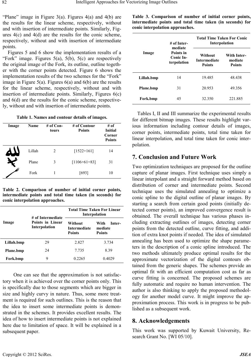

Intelligent Approaches for Vectorizing Image Outlines
82
“Plane” image in Figure 3(a). Figures 4(a) and 4(b) are
the results for the linear scheme, respectively, without
and with insertion of intermediate points. Similarly, Fig-
ures 4(c) and 4(d) are the results for the conic scheme,
respectively, without and with insertion of intermediate
points.
Figures 5 and 6 show the implementation results of a
“Fork” image. Figures 5(a), 5(b), 5(c) are respectively
the or igi nal i mage of t he For k, its outline, o utline toget h-
er with the corner points detected. Figure 6 shows the
implementation results of the two schemes for the “Fork”
image in F ig ure 5 (a). Figures 6(a) and 6(b) are the results
for the linear scheme, respectively, without and with
insertion of intermediate points. Similarly, Figures 6(c)
and 6 (d) are the results for the conic scheme, respective-
l y, w i t hout and with insertion of inter mediate points.
Table 1. N ames and contour details of images.
Image
Name
# of Con-
tours
# of Contour
Points
# of
Initial
Corner
Points
Lillah 2 [1522+161] 14
Plane 3 [1106+61+83] 31
Fork 1 [693] 10
Table 2. Comparison of number of initial corner points,
intermediate points and total time taken (in seconds) for
conic interpo lation approache s.
Image # of Intermediate Points in Linear
Interpolation
Total Time Taken For Linea r
Interpolation
Without
Intermediate
Points
With Inter-
mediate
Points
Lillah.bmp 29 2.827 3.734
Plane.bmp 24 7.735 8.39
Fork.bmp 9 0.2265 0.4029
One can see that the approximation is not satisfac-
tor y whe n i t i s a c hie ved over t he co r ner p o int s onl y. This
is specifically due to those segments which are bigger in
size and highly curvy in nature. Thus, some more treat-
ment i s requi red fo r such o utline s. Thi s is the reaso n that
the idea to insert some intermediate points is demon-
strated in the schemes. It provides excellent results. The
idea of how to insert intermediate p oints is not explained
here due to limitation of space. It will be explained in a
subsequent paper.
Table 3. Comparison of number of initial corner points,
intermediate points and total time taken (in seconds) for
conic inte rpolatio n approac hes.
Image
# of Inter-
mediate
Points in
Conic In-
terpolation
Total Time Taken For Conic
Interpolation
Without
Intermediate
Points
With Inter-
mediate
Points
Lillah.bmp 14 19.485 48.438
Plane.bmp 31 20.953 49.356
Fork.bmp 45 32.350 221.885
Tables I, II and III summarize the experimental results
for different bitmap images. These results highlight var-
ious information including contour details of images,
corner points, intermediate points, total time taken for
linear interpolation, and total time taken for conic inter-
polation.
7. Conclusion and Future Work
Two optimization techniques are proposed for the outline
capture of planar images. First technique uses simply a
linear interpolant and a straight forward method based on
distribution of corner and intermediate points. Second
technique uses the simulated annealing to optimize a
conic spline to the digital outline of planar images. By
starting a search from certain good points (initially de-
tected corner points), an improved convergence result is
obtained. The overall technique has various phases in-
cluding extracting outlines of images, detecting corner
points from the detected outline, curve fitting, and addi-
tion of extra knot points if needed. The idea of simulated
annealing has been used to optimize the shape parame-
ters in the description of a conic spline introduced. The
two methods ultimately produce optimal results for the
approximate vectorization of the digital contours ob-
tained from the generic shapes. The schemes provide an
optimal fit with an efficient computation cost as far as
curve fitting is concerned. The proposed sc h eme s are
fully automatic and require no human intervention. The
author is also thinking to apply the proposed methodol-
ogy for another model curve. It might improve the ap-
proximation process. This work is in progress to be pub-
lished as a subsequent work.
8. Acknowledgements
This work was supported by Kuwait University, Re-
search Grant No. [WI 05/10].

Intelligent Approaches for Vectorizing Image Outlines
83
REFERENCES
[1] D. Chetrikov, S. Zsabo, “A Simple and Efficient Algo-
rithm for Detection of High Curvature Points in Planar
Curves”, Proceedings of the 23rd Workshop of the Aus-
tralian Pattern Recognition Group, 1999, pp. 1751-2184.
[1] A. A. Goshtasby, “Grouping and Parameterizing Irregu-
larly Spaced Points for Curve Fitting”, ACM Transac-
tions on Graphics, Vol. 19 , No. 3, 2000, pp. 185-203.
[2] P. Reche, C. Urdiales, A. Bandera,C. Trazegnies, F.
Sandoval, “Corner Detection by Means of Contour Local
Vectors”, Electronic Letter s, Vol. 38, No. 14, 2002.
[3] M. Marji, P. Siv, “A New Algorithm for Dominant Points
Detection and Polygonization of Digital Curves”, Pattern
Recognition, 2003, p p. 22 39-2251.
[4] Wu -Chih Hu, “Multiprimitive Segmentation Based on
Meaningful Breakpoints for Fitting Digital Planar Curves
with Line Segments and Conic Arcs”, Image and Vision
Computing, 2005, pp. 783-789.
[5] H. Freeman, L. S. Davis, “A corner finding algorithm for
chain-coded curves”, IEEE Trans. Computers, Vol. 26,
1977, pp . 297-303.
[6] N. Richard, T. Gilbert, “Extraction of Dominant Points
by estimation of the contour fluctuations”, Pattern Rec-
ognition, Vol. 35, 2002, pp. 1447-1462.
[7] M. Sarfraz, “Representing Shapes by Fitting Data using
an Evolutionary Approach”, International Journal of
Computer-Aided Design & Applications, Vol. 1, No. 1-4,
2004, pp 179-186.
[8] M. Sarfraz, M. A. Khan, “An Automatic Algorithm for
Approximating Boundary of Bitmap Characters”, Future
Generation Computer Systems, 2004, pp. 13 27-1336.
[9] M. Sarfraz, “Some Algorithms for Curve Design and
Automatic Outline Capturing of Images”, International
Journal of Image and Graphics, 2004, pp. 301-324.
[10] Z. J. Hou, G. W. Wei, “A New Approach to Edge Detec-
tion”, Pattern Recognition, 2002, pp. 1559-1570.
[11] M. Sarfraz, “Computer-Aided Reverse Engineering using
Simulated Evolution on NURBS”, International Journal
of Virtual & Physical Prototyping, Vol. 1, No. 4, 2006,
pp. 243 – 257.
[12] M. Sarfraz, M. Riyazuddin, M. H. Baig, “Capturing Pla-
nar Shapes by Approximating their Outlines, Internation-
al Journal of Computational and Applied Mathematics,
Vol. 189, No. 1-2, 2006, pp. 49 4 – 512.
[13] M. Sarfraz, A. Rasheed, “A Randomized Knot Insertion
Algorithm for Outline Capture of Planar Images using
Cubic Spline”, The Proceedings of The 22th ACM
Symposium on Applied Computing (ACM SAC-07), Seoul,
Korea, 2007 , p p. 71 – 75.
[14] H. Kano , H. Nakata, C. F . Martin, “Optimal Curve Fitting
and Smoothing using Normalized Uniform B-Splines: A
Tool for Studying Complex Systems”, Applied Mathe-
matics and Computation, 2005, pp. 96 -128.
[15] Z. Yang, J. Deng, F. Chen, “Fitting Unorganized Point
Clouds with Active Implicit Spline Curves”, B- Visual
Computer, 2005, pp. 831-839.
[16] G. Lavoue, F. Dupont, A. Baskurt, “A New Subdivision
Based Approach for Piecewise Smooth Approximation of
3D Polygonal Curves”, Pattern Recognition, Vol. 38,
2005, pp . 1139-1151.
[17] H. Yang, W. Wang, J. Sun, “Control Point Adjustment
for B-Spline Curve Approximation”, Computer Aided
Design, Vol. 36, 2004, pp. 639-652.
[18] J. H. Horng, “An Adaptive Smoothing Approach for Fit-
ting Digital Planar Curves with Line Segments and Cir-
cular Arcs ”, Pattern Recog ni tion Letters, Vol. 2 4, No. 1-3,
2003, pp . 565-577.
[19] B. Sarkar, L. K. Singh, D. Sarkar, “Approximation of
Digital Curves with Line Segments and Circular Arcs us-
ing Genetic Algorithms”, Pattern Recognition Letters,
Vol. 24, 2003 , pp. 25 85-2595.
[20] X. Yang, “Curve Fitting and Fairing using Conic Spines”,
Computer Aided Design, Vol. 6, No. 5, 2004, pp.
461-472.
[21] X. N. Yang, G. Z. Wang “Planar Point Set Fairing and
Fitting by Arc Splines”, Computer Aided Design, 2001,
pp. 35-43.
[22] M. Sarfraz, “Designing Objects with a Spline”, Interna-
tional Journal of Computer Mathematics, Vo l. 85, No . 7,
2008.
[23] S. Kirkpatrick, C. D. Gelatt Jr., M. P. Vecchi, "Optimiza-
tion by Simulated Annealing", Science, Vol. 220, No
4598, 1983, pp. 671-680.
[24] R. C. Gonzalez, R. E. Woods, S. L. Eddins, “Digital Im-
age Processing Using MATLAB”, 2nd Ed., 2009, Gates-
mark Publishing.
[25] M. S. Nixon, A.S. Aguado, “Feature extract ion and image
processing”, 2008, Elsevier.
[26] M. Sarfraz, “Outline Capture of Images by Multilevel
Coordinate Search on Cubic Splines”, Lecture Notes in
Artificial Intelligence, A. Nicholson and X. Li (Eds.):
LNAI 5866, Springer-Ver lag Berl in Heid elber g, 2009, pp.
636–645.
[27] M. Sarfraz, “Vectorizing Outlines of Generic Shapes by
Cubic Spline using Simulated Annealing”, International
Journal of Computer Mathematics, Vol. 87, No. 8, 2010,
pp. 1736 – 1751.
[28] Sarfraz, M. (2011), Capturing Image Outlines using
Simulated Annealing Approach with Conic Splines,The
Proceedings of The International Conference on
Information and Intelligent Computing (ICIIC 2011),
Hong Kong, China, November 25-27, 2011, IPCSIT Vol.
18, pp. 152 – 157, IASCIT Press Singapore.
[29] M. Sarfraz, “Vectorizing Image Outlines using Spline
Computing Approach”, The Proceedings of The 4th In-
ternational Conference on Machine Learning and Com-
puting (ICMLC 2012), Hong Kong, China, 2012, ASME
Press.