13
Technology and Investment, 2013, 4, 78-82
Published Online Febr uary 20 http://www.SciRP.org/journal/ti)
Copyright © 20 SciRes. TI
Heterogeneous Fleet Vehicle Routing Problem with Selec-
tion of Inter-Depots
ČIČKOVÁ Zuzana, PEKÁR Juraj, BREZINA Ivan, REIFF Marian
Department of Operations Research and Econometrics, University of Economics, Bratislava, Slovakia
Email : pekar @euba.sk
Received 2012
ABSTRACT
The paper presents heterogeneous fleet vehicle routing problem with selection of inter-depots. The goal of the proposed
model is to schedule shipments of goods from the central depot to the inter-depots and finally to the endpoint customers,
so that as inter-depots are considered the existing capacities of endpoints customers. In given type of transportation it
can be expected to use two types of vehicles: large capacity vehicles ensuring the distribution of goods from the central
ware ho use and small capacity vehicles ensuring the delivery of goods from inter-depots for late shipment to other cus-
tomers. The principle of the model is illustrated on three demonstrative instances
Keywords: mult i -depot vehicle routing problem; replenishment; mathematical programming
1. Introduction
The problem that addresses the distribution of goods from
a central warehouse to various delivery points using a
fleet of vehicle with limited capacity is known as capa-
cited vehicle routing problem (CVRP). The relevance of
that problem follows from many published articles, and
also fro m practical applications of distribution (e. g. [1],
[2], [ 3], [ 8]). The CVRP belongs to the group of NP-hard
problems, so the possibility of solution of above men-
tioned problem is studied by many authors. Nowadays
research attention is focused on heuristics, for example,
the evolutionary approach is proposed by in [2], [3], [4],
[5], [6], [7]. The problem can be extended by adding in-
ter-depots to the central storage facilitie s and also by
considering the use of multiple types of vehicles ([6] , [8],
[9], [10], [11], [12]). Delivery is then realized in two
levels, the first level is to carry the goods from a central
distribution warehouse into inter-depots and the second
level implements the tr an s s hi p me nt of goods to the end-
point customers. Generally, each facilit y tends to be ex-
actly defined to belong to the group of inter-depots or to
the group of final customers. However, in nowadays real
life situations, companies that are dealing with this type of
distribution do not open new inter-depots, which opening
is associated with the construction cost and subsequently
with operation cost, but they utilize endpoint customers
useful storage capacities also as an intermediate storage
for late shipment to other customers. In this case, as in-
ter-depots stor a ge are used existing capacities of end-
points customers, so that existing supply points may or
may not also serve as a inter-depots. In given type of
problem it can be expected to use two types of vehicles:
large capacity vehic le s (L) ensuring the distribution of
goods from the central warehouse and smal l capacity
vehic l es (S) ensuring the delivery of goods from in-
ter-depots and also from central warehouse. In this paper
we formulate the considered problem as a mat h ematical
programming model later used for further analysis. Due to
its computational complexity, the formulated problem is
solvable by classical optimization techniques (as well as
other modifications of CV RP ) only for small instances.
We chose the following structure of the paper: In the first
part we present classical CVRP, because it forms a base of
modeling for a wide variety of routing problems. The next
section describes the construction of proposed heteroge-
neous fleet vehicle routi ng problem with selection of
inter-depots. Afterwards, the obtained experimental re-
sults are given and discussed. In this section, we also
analyze presented model under different vehicle cost.
2. Capacited Vehicle Routing Problem
Classical capacitated vehicle routing problem is the basic
routing model and it can be stated as follows: Let
G = (V, E) be the full weighted graph, where V represents
set of n nodes and E represents n.n set of edges. The node
v1 represents the location of central warehouse and the
nodes vi = 2, 3, ...n represent location of endpoint cus-
tomers.
Assumptions of CVRP:
• Unlimited number of vehicles with a certain capacity g,
which are located in a certain depot with unlimited ca-
pacity.
13 (

Č. Zuzana ET AL.
TI
• Set of delivery points (endpoi nts) with a certain de-
man d bi, i = 2, 3, ...n (the orders have to be delivered in
full).
• Minimal distances between all the pairs of endp oint s
customers and also between the endpoint customers
and the depot are known (matrix D).
• The goal is to fi nd optimal vehicle routes (so that the
total distance traveled is minimized) in such a way that
each customer is visited only once by exactly one ve-
hicle, all routes start and end at the depot, and the total
demands of all customers on one particular route must
not exceed the capacity of the vehicle.
• In the model is implicitly assumed bi ≤ g for each
i = 2, 3, ...n.
Parameters
D – matrix of minimal distances between all the pairs of
nodes
c – transportation cost per unit
b – vector of demands
g – capacity of the vehic le .
Variables
{ }
0, 1
ij
x∈
,
, 1, 2, ...ij n=
- binary variables, that
represent the use of corresponding edge: If the edge (i,j)
is on the route of the some vehicle 1
ij
x=
, otherwise
0
ij
x=
,
0
i
u≥, 1, 2, ...in= - non-negative variables, that
represent the cumulative demand of the individual nodes
on the route of any vehicl e.
Starting value of variable
1
0u=
CVRP formulation can be interpreted as follows:
( )
11
min
nn
ij ij
ij
fc dx
= =
= →
∑∑
X, u
Objective function ensures minimization of total tran s-
portation costs of vehicles.
1
1
=
∑
=
n
i
ij
x
, 2, 3, ...jn= , ij≠
The equations represent that the vehicle comes to each
node (except the centre) exactly once.
1
1
=
∑
=
n
j
ij
x
, 2, 3, ...in= , ij≠
The equations represent that the vehicle leaves each node
(except the centre) exactly once.
( )
0
ijj ij
u bux+− =
, 1, 2,...in= ,
2, 3,...jn=
,
ij≠
ii
bu g≤≤
, 2, 3, ...in=
The equations are anti-cyclic constraints which ensure
also the accumulation of the load of the vehicle in such
way the load must not exceed the vehicle capacity.
3. Heterogeneous Fleet Vehicle Routing
Problem with Selection of Inter-Depots –
Problem Formulation
The model was in general introduced by authors in [13].
Problem is useful for company dealing with one central
warehouse (edge v1 denotes localization of the central
ware ho use ) and n – 1 delivery points. The large capacity
vehicles L are available in the central warehouse. The
small capacity vehicles S are available at the endpoints
and also at the central warehouse. Transportation costs
per unit are known for both types of vehicles . It is as-
sumed the known demand of all delivery points. All the
orders have to be delivered in full. Each of the n – 1
delivery point can be used as a inter-depot, so demand of
other d elivery point can be can be met from the in-
ter-depot by vehicle S. The route of vehicle S can be fi-
nished also in other than starting inter-depot, (either cen-
tral warehouse can be assumed to serve as inter-depot),
but the number of incoming and outc omin g vehicles of
type S must be identical.
Parameters
D – matrix of minimal distances between all the pairs of
nodes
b – vector of demands
gL – capacity of the vehicle L
gS – capacity of the vehicle S
cL – cost per unit of the vehicle L
cS – cost per unit of the vehicle S .
4. Heterogeneous Fleet Vehicle Routing
Problem with Selection of Inter-Depots –
Model
Variables
{ }
0, 1
ij
x∈
,
, 1, 2, ...ij n=
- binary variables, that
represent the use of corresponding edge by vehicle L: If
the edge (i,j) is on the route of the vehicle L 1
ij
x= , oth-
erwis e
0
ij
x=
.
{ }
0, 1
ij
y∈
,
, 1, 2, ...ij n=
- binary variables, that
represent the use of corresponding edge by vehicle S: If
the edge (i,j) is on the route of the vehicle S 1
ij
y= ,
otherwi s e 0
ij
y= .
0
ij
yy ≥
,
, 1, 2, ...ij n=
- non-negative variables, that
represent the cumulat i ve amount of unloaded goods
transported on the edge (i,j).
79
13 Copyright © 20 SciRes.

Č. Zuzana ET AL.
TI
0
i
u≥,1, 2, ...in= - non-negative varia bles, that
represent the cumulative demand of the individual nodes
on the route of vehicle L (including eventual distrib ution
with a vehicles S from corresponding node).
0
i
z≥,
1, 2, ...in=
- non-negative variables, that
represent t he cumulative demand of the individual nodes
on the route of vehicle S.
0
i
w≥ , 2, 3, ...in= - non-negative variables, that
represent the quantity of goods that is distributed from
corresponding node by vehicl e S.
0
i
q≥, 1, 2, ...in= - non-negative variables, that
represent the quantity of imported goods to the corres-
ponding node by a vehicle L.
Starting values of variables
11
1x=
0
ii
x=
, 2, 3, ...in=
1
0u=
1
0z=
The model can be interpreted as follows:
( )
11 11
, min
nn nn
Lij ijSijij
ij ij
fcdx cdy
= == =
=+→
∑∑ ∑∑
X,Y,YY,u,z w,q
Objective function ensures minimization of total tran s-
portation costs for vehicles L and vehicles S.
1
1
n
ij
i
x
=
≤
∑
,
2, 3, ...jn=
,
ij≠
The equations represent that the vehicle L comes to each
node (except the centre) no more than once.
1
1
n
ij
j
x
=
≤
∑,
2, 3, ...in=
,
ij≠
The equations represent that the vehicle S leaves to each
node (except the centre) no more than once.
11
nn
ij ji
jj
xx
= =
=
∑∑
,
1, 2, ...in=
,
ij≠
The equations represents that the number of a rriva ls and
exits of ve hic le L into and from the node is identical.
( )
.0
ijjij
uqux+− =
, 1, 2, ...in= ,
2, 3, ...jn=
,
ij≠
The equations provide the accumulation of the load of
the vehicle L.
iL
ug≤
, 2, 3, ...in=
The equations represent that the capacity of vehicle L
must not be exceeded.
11
nn
ii
ii
qb
= =
=
∑∑
The equation represents that the demand of all nodes
have to be met.
1
1., 2,3,...
n
ij ii
j
x bzin
=

− ≤=


∑
The equations provide the balance of variables (starting
value s for a vehicle S) in the case node serves as an in-
ter-depot.
11
0, 2,3,...
nn
ij ji
ii
ij
xyjn
= =
≠



− +≥=





∑∑
The equations represent the self-service of the node, in
the case the node is on the route of a vehicle L.
1
1
n
ij
j
y
=
≥
∑
,
1, 2, ...in=
The equations represent that each node must be served.
11
nn
ij ji
jj
yy
= =
=
∑∑
,
1, 2, ...in=
,
ij≠
The equations rep resent that the number of incoming and
the number of outcoming routes in and out of the node is
identical.
( )
1
. .(1)0
n
jii ijsj
s
z bzyx
=
+−− =
∑
, 1, 2, ...in= ,
2, 3, ...jn=
,
ij≠
The equations provide the accumulation of the load of
the vehicle S.
iS
zg≤
, 1, 2, ...in=
The equations represent that the capacity of vehicle S
must not be exceeded
1
n
ii iij
j
w qbx
=
= −⋅
∑,
2, 3, ...in=
The equations represent the balance of quantity of goods
of vehicl e S.
11
.
nn
jiij j
ii
ij
yyx w
= =
≠
=
∑∑ ,
2, 3, ...jn=
The equations provide that the amount of goods for ve-
hicles S cannot exceed the quantity of goods that is
transported into the node by a vehicle L.
.
ji jii
yy yz=
,
, 1, 2, ...ij n=
,
ij≠
The equations provide the balance of cumulative number
of unloaded goods transported on the edge (i, j).
{ }
0, 1
ij
y∈, , 1, 2, ...ij n=
{ }
0, 1
ij
x∈
,
, 1, 2, ...ij n=
0
ij
yy ≥
,
, 1, 2, ...ij n=
0
i
u≥,
1, 2, ...in=
0
i
w≥
, 2, 3, ...in=
0
i
z≥,
1, 2, ...in=
0
i
q≥, 1, 2, ...in=
5. Empirical Results
The principle of heterogeneous fleet vehicle routing
problem with selection of inter-depots is illustrated on
80
13 Copyright © 20 SciRes.

Č. Zuzana ET AL.
TI
three de monstrative instances. Firstly, cost per vehicle L
and vehicle S were considered in proportion ten to six,
L (10), S (6 ). Later, in order to demonstrate the model
functionality, it was considered to set significantly higher
costs per vehicle L, (value 100) and to set significa nt l y
lower costs per vehicle S (value 1). This should lead to
preference of vehicles S (if it is possible to fulfill the de-
mands due to the restriction limit of the vehicle). In the
third case, high cost fo r vehicle S (100) and low cost for
vehicle L (1) were preferred, which should essentially
resul t s in the preference of vehicle L, i.e. the model
works as classical CVRP.
Model input data, used in all three demonstrative in-
stances:
n – number of nodes = 10
b – vector of demands = (0, 5, 2, 2, 20, 10, 6, 3, 9, 10)
gL – capacity of the vehicle L = 50
gS – capacity of the vehicle S = 15
D – matrix of minimal distances between all the pairs of
nodes (Table 1)
Table 1
For each demonstrative instance the input data were
modified in different cost adjustments:
1) Proportional costs adjustment:
cL – cost per unit of the vehicle L = 10
cS – cost per unit of the vehic le S = 6
2) The higher cost of operating a large capacity vehicle
compared to a small capacity vehicles:
cL – cost per unit of the vehicle L = 100
cS – cost per unit of the vehic le S = 1
3) The higher cost of operating a small capacity vehicles
compared to a large capacity vehicle:
cL – cost per unit of the vehicle L = 1
cS – cost per unit of the veh ic le S = 1 00
Proposed problems were solved using software GAMS.
Solutions of the model for various demonstrative in-
stances:
1. Insta nc e with proportional cost values (cL = 10, cS =
6). Computed value f = 9103.8. Solution is depicted
on Figure 1, dashed lines represent the transportation
by vehicle L, and full line represents the route of ve-
hicles S.
Figure 1
2. Insta nc e with significantly higher cost of operating
vehicle L (cL = 100, cS = 1). Computed value f =
17757.5. Solution is depicted on Figure 2, dashed
lines represent the route of vehicle L and full lines
represent the route of vehicles S. The value of objec-
tive function f has significantly increased. It is
caused by the fact that delivery cannot be made only
by vehicle type S because of the demand of node 5
exceeds the capacity of the vehicle S. At the same
time, assumption that the vehicle S can finish its
rout e in other as in starting i nt er -depot is met, how-
ever the number of incoming and outgoing vehicles
of type S must be identical (node 1 and 5).
Figure 2
3. Case with significantly higher cost of operating ve-
hicles S (cL = 1, cS = 100). Computed value f =
1152.2. Solution is depicted on Figure 3. Dashed
lines represent the transportation by L type vehicle,
D12345678910
10 11148.5 216.782.5 207.840.8 182.5 105.1 118.8
2111 077.5 301.633.5 125.9 151.88078.9 121.9
348.5 77.50265.267 169.289.3137.5 132.2 145.9
4216.7 301.6 265.20273.1424.5 182.1 374.5 259.1272.8
582.533.567 273.10151.4123.3105 79.1 93.4
6207.8 125.9 169.2 424.5 151.40248.691.5 184.4 228.1
740.8 151.889.3 182.1 123.3 248.60223.3 145.9159.6
8182.580137.5 374.510591.5 223.30117.9 161.6
9105.178.9 132.2 259.179.1 184.4 145.9 117.9046.2
10 118.8 121.9 145.9 272.893.4 228.1 159.6161.646.20
1
6
4
8
5
9
3
10
7
2
1
3
4
6
5
9
8
2
7 10
81
13 Copyright © 20 SciRes.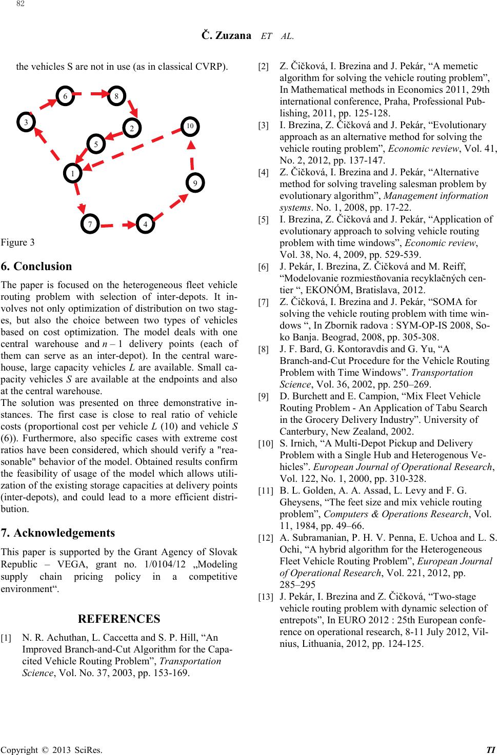

Č. Zuzana ET AL.
TI
1
3
4
6
5
8
7
2 10
9
the vehicles S are not in use (as in classical CVRP).
Figure 3
6. Conclusion
The paper is focused on the heterogeneous fleet vehicle
routing problem with selection of inter -depots. It in-
volves not only optimization of distribution on two stag-
es, but also the choice between two types of vehicles
based on cost optimization. The model deals with one
central warehouse and n – 1 delivery points (each of
them can serve as an inter-depot). In the central ware-
house, large capacit y vehicles L are available. Small ca-
pacity vehicles S are available at the endpoints and also
at the central warehouse.
The solution was presented on three demonstrative in-
stance s. The first case is close to real ratio of vehicle
costs (proportional cost per vehicle L (10) and vehicle S
(6)). Furthermore, also specific cases with extreme cost
ratios have been considered, which should verify a "rea-
sonable" behavior of the model. Obtained results confirm
the feasibility of usage of the model which allows utili-
zation of the existing storage capacities at delivery points
(inter-depots), and could lead to a more efficient distri-
butio n.
7. Acknowledgements
This paper is supported by the Grant Agency of Slovak
Republic – VEGA, grant no. 1/0104/12 „Modeling
supply chain pricing policy in a competitive
environ ment“.
REFERENCES
[1] N. R. Achuthan, L. Caccetta and S. P. Hill, “An
Improved Branch-and-Cut Algorithm for the Capa-
cited Vehicle Routing Problem”, Transportation
Science, Vol. No. 37, 2003, pp. 153-169.
[2] Z. Čičková, I. Brezina and J. Pekár, “A memetic
algorithm for solving the vehicle routing problem”,
In Mathematical methods in Economics 2011, 29th
international conference, Praha, Professional Pub-
lishing, 2011, pp. 125-128.
[3] I. Brezina, Z. Čičko vá a nd J. Pekár, “Evolutionary
approach as an alternative method for solving the
vehicle routing problem”, Economic review, Vol. 41,
No. 2, 2012, pp. 137-147.
[4] Z. Čičková, I. Brezina and J. Pekár, “Alternative
method for solving traveling salesman problem by
evolut iona r y algorithm”, Management information
system s. No. 1, 2008, pp. 17-22.
[5] I. Brezina, Z. Čičko vá a nd J. Pekár, “Application of
evolutionary approach to solving vehicle routing
problem with time windows”, Economic review,
Vol. 38, No. 4, 2009, pp. 529-539.
[6] J. Pekár, I. Brezina, Z. Čičková and M. Reiff,
“Modelovanie rozmiestňovania recyklačných cen-
tier “, EKONÓM, Bratisla va, 2012.
[7] Z. Čičková, I. Brezina and J. Pekár, “SOMA for
solving the vehicle routing problem with time win-
dows “, In Zbornik radova : SYM-OP-IS 2008, So-
ko Banja. Beograd, 2008, pp. 305-308.
[8] J. F. Bard, G. Kontoravdis and G. Yu, “A
Branch-and-Cut Procedure for the Vehicle Routing
Problem with Time Windows”. Transportation
Science, Vol. 36, 2002, pp. 250–269.
[9] D. Burchett and E. Campion, “Mix Fleet Vehicle
Routing Problem - An Application of Tabu Search
in the Grocery Delivery Industry”. University of
Canterbury, New Zealand, 2002.
[10] S. Irnich, “A Multi-Depot Pickup and Delivery
Problem with a Single Hub and Heterogenous Ve-
hicles”. European Journal of Operational Research,
Vol. 122, No. 1, 2000, pp. 310-328.
[11] B. L. Golden, A. A. Assad, L. Levy and F. G.
Gheysens, “The feet size and mix vehicle routing
problem”, Computers & Operations Research, Vol.
11, 1984, pp. 49–66.
[12] A. Subramanian, P. H. V. Penna, E. Uchoa and L. S.
Ochi, “A hybrid algorithm for the Heterogeneous
Fleet Vehicle Routing Problem”, European Journal
of Operational Research, Vol. 221, 2012, pp.
285–295
[13] J. Pekár, I. Brezina and Z. Čičko vá , “Two-stage
vehicle routing problem with dynamic selection of
entrepots”, In EURO 2012 : 25th European confe-
rence on operational research, 8-11 July 2012, Vil-
nius, Lithuania, 2012, pp . 124-125.
82
13 Copyright © 20 SciRes.