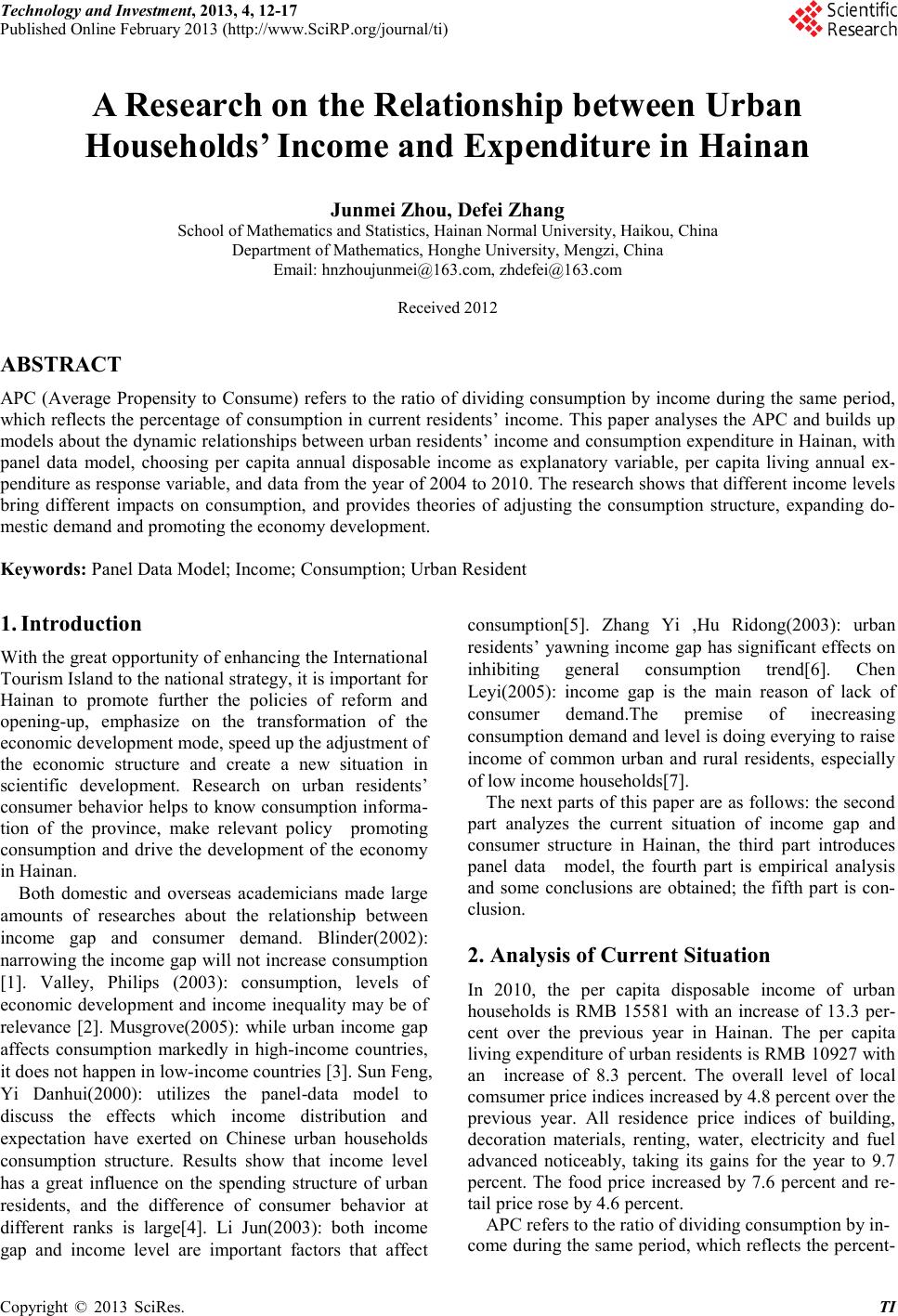Technology and Investment, 2013, 4, 12-17
Published Online February 2013 (http://www.SciRP .org/journal/ti)
A Research on the Relationship between Urban
Households’ Income and Expenditure in Hainan
Junmei Zhou, Defei Zhang
School of Mathematics and Statistics, Hainan Normal University, Haikou, China
Department of Mathematics, Honghe University, Mengzi, China
Received 2012
ABSTRACT
APC (Average Propensity to Consume) refers to the ratio of dividing consumption by income during the same period,
which reflects the percentage of consumption in current residents’ income. This paper analys es the APC and builds up
models about the dynamic relationships between urban residents’ income and consumption expenditure in Hainan, with
panel data model, choosing per capita annual disposable income as explanatory variable, per capita living annual ex-
penditure as response variable, and data from the year of 2004 to 2010. The research shows that different income levels
bring different impacts on consumption, and provides theories of adjusting the consumption structure, expanding do-
mest i c demand and promoting the economy development.
Keywords: Panel Data Model; Income; Cons u mp t io n; Urban Resi d ent
1. Introduction
With the great opportunity of enhancing the International
Tourism Island to the national strategy, it is important for
Hainan to promote further the policies of reform and
ope ni ng -up, emphasize on the transformation of the
economic development mode, speed up the adjustment of
the economic structure and create a new situation in
scientific development. Research on urban residents’
consumer behavior helps to know consumption informa-
tion of the province, make relevant policy promoting
consumption and drive the development of the economy
in Hainan.
Both domestic and overseas academicians made large
amounts of researches about the relationship between
in come gap and consumer demand. Blinder(2002):
narrowing the income gap will not increase consumption
[1]. Valley, Philips (2003): consumption, levels of
economic development and income inequality may be of
relevance [2]. Musgrove(2005): while urban income gap
affects consumption markedly in high-income countries,
it does not happen in low-income countries [3]. Sun Feng,
Yi Danhui(2000): utilizes the panel-data model to
discuss the effects which income distribution and
expectation have exerted on Chinese urban households
consumption structure. Results show that income level
has a great influence on the spending structure of urban
residents, and the difference of consumer behavior at
different ranks is large[4]. Li Jun(2003): both income
gap and income level are important factors that affect
consumption[5]. Zhang Yi ,Hu Ridong(2003): urban
residents’ yawning income gap has significant effects on
inhibiting general consumption trend[6]. Chen
Leyi(2005): income gap is the main reason of lack of
consumer demand.The premise of inecreasing
consumption demand and level is doing everying to raise
income of common urban and rural residents, especially
of low income households[7].
The next parts of this paper are as follows: the second
part analyzes the current situation of income gap and
consumer structure in Hainan, the third part introduces
panel data model, the fourth part is empirical analysis
and some conclusions are obtained; the fifth part is con-
clusion.
2. Analysis of Current Situation
In 2010, the per capita disposable income of urban
households is RMB 15581 with an increase of 13.3 per-
cent over the previous year in Hainan. The per capita
living expenditure of urban residents is RMB 10927 with
an increase of 8.3 percent. The overall level of local
comsumer price indices increased by 4.8 percent over the
previous year. All residence price indices of building,
decoration materials, renting, water, electricity and fuel
advanced noticeably, taking its gains for the year to 9.7
percent. The food price increased by 7.6 percent and re-
tail price rose by 4.6 percent.
APC refers to the ratio of dividing consumption by in-
come during the same period, which reflects the percent-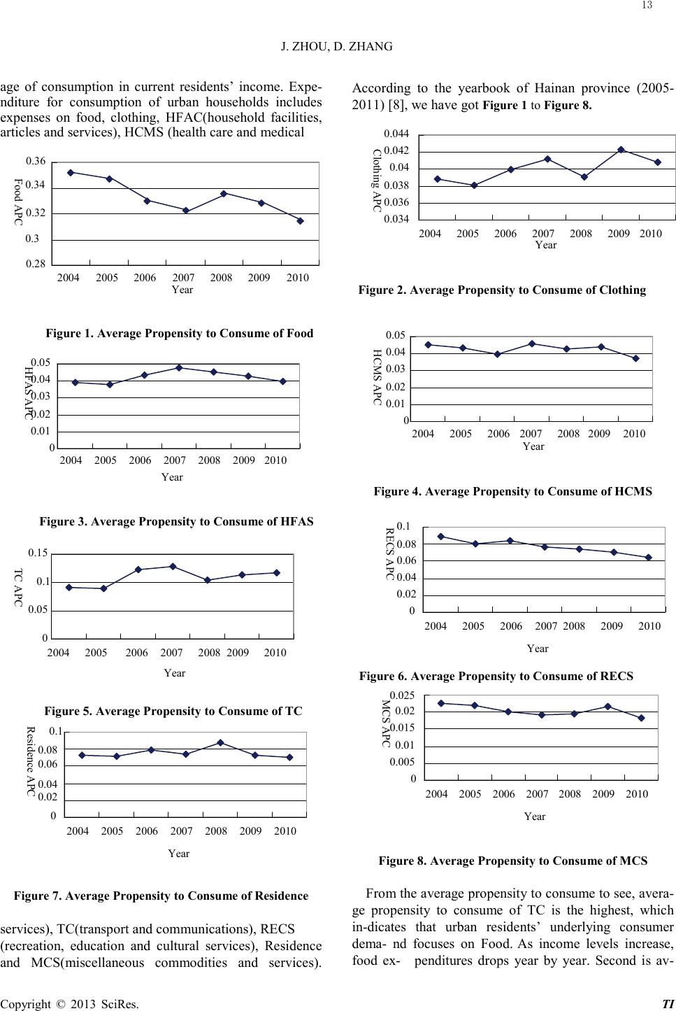

J. ZHOU, D. Z HANG
age of consumption in current residents’ income. Expe-
nditure for consumption of urban households includes
expenses on food, clothing, HFAC(household facilities,
articles and services), HCMS (health care and medical
Figure 1. Average Propensity to Consume of Food
Figure 3. Average Propensity to Consume of HFAS
Figure 5. Average Propensity to Consume of TC
Figure 7. Average Propensity to Consume of Residence
services), TC(transport and communicatio ns), RE CS
(recreation, education and cultural services), Residence
and MCS(miscellaneous commodities and services).
According to the yearbook of Hai nan province (2005-
2011) [8], we have got Figure 1 to Fi gure 8.
Figure 2. Average Propensity to Consume of Clothing
Figure 4. Average Propensity to Consume of HCMS
Figure 6. Average Propensity to Consume of RECS
Figure 8. Average Propensity to Consume of MCS
From the average propensity to consume to see, avera-
ge propensity to consume of TC is the highest, which
in-dicates that urban residents’ underlying consumer
dema- nd focuses on Food. As income levels increase,
food ex- penditures drops year by year. Second is av-
0.034
0.036
0.038
0.04
0.042
0.044
2004
2005
2006
2007
2008
2009
2010
Year
Clothing APC
0
0.005
0.01
0.015
0.02
0.025
2004
2005
2006
2007
2008
2009
2010
Year
MCS APC
0
0.02
0.04
0.06
0.08
0.1
2004
2005
2006
2007
2008
2009
2010
Year
Residence APC
0
0.02
0.04
0.06
0.08
0.1
2004
2005
2006
2007
2008
2009
2010
Year
RECS APC
0
0.01
0.02
0.03
0.04
0.05
2004
2005
2006
2007
2008
2009
2010
Year
HCMS APC
0
0.01
0.02
0.03
0.04
0.05
2004
2005
2006
2007
2008
2009
Year
HFAS APC
2010
0
0.05
0.1
0.15
2004
2005
2006
2007
2008
2009
2010
Year
TC APC
0.28
0.3
0.32
0.34
0.36
2004
2005
2006
2007
2008
2009
2010
Food APC
Year
13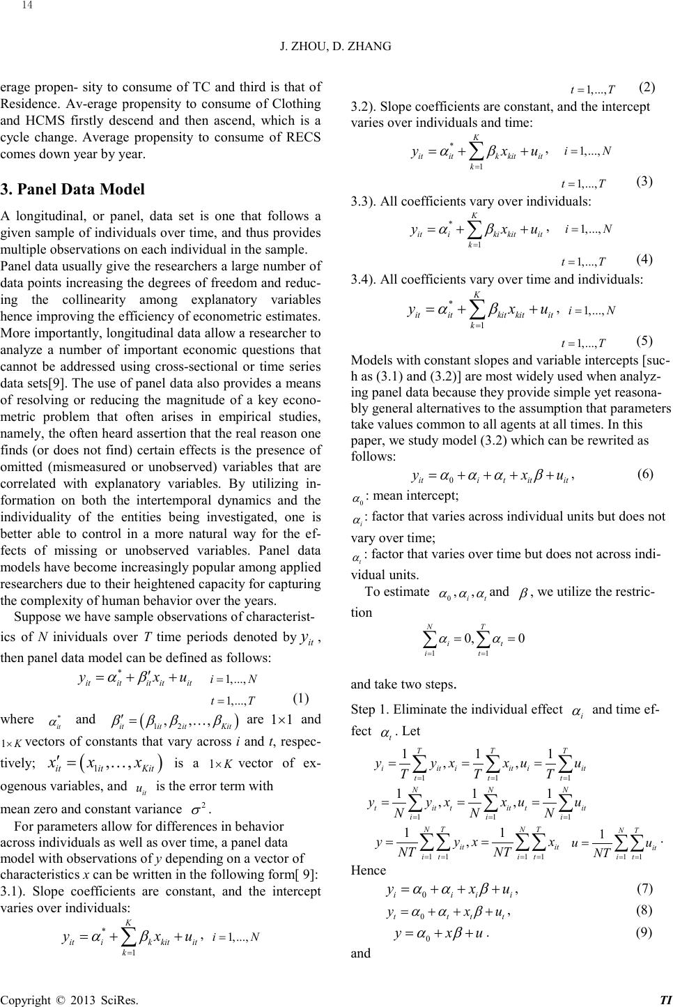

J. ZHOU, D. Z HANG
erage propen- sity to consume of TC and third is that of
Residence. Av-erage propensity to consume of Clothing
and HCMS firstly descend and then ascend, which is a
cycle change. Average propensity to consume of RECS
comes down year by year.
3. Panel Data Model
A longitudinal, or panel, data set is one that follows a
given sample of individuals over time, and thus provides
multiple observations on each individual in the sample.
Panel data usually give the researchers a large number of
data points increasing the degrees of freedom and reduc-
ing the collinearity among explanatory variables
hence improving the efficiency of econometric estimates.
More importantly, longitudinal data allow a researcher to
analyze a number of important economic questions that
cannot be addressed using cross-sectional or time series
data sets[9]. The use of panel data also provides a means
of resolving or reducing the magnitude of a key econo-
metric problem that often arises in empirical studies,
namely, the often heard assertion that the real reason one
finds (or does not find) certain effects is the presence of
omitted (mismeasured or unobserved) variables that are
correlated with explanatory variables. By utilizing in-
formation on both the intertemporal dynamics and the
individuality of the entities being investigated, one is
better able to control in a more natural way for the ef-
fects of missing or unobserved variables. Panel data
models have become increasingly popular among applied
researchers due to their heightened capacity for capturing
the complexity of human behavior over the years.
Suppose we have sample observations of characterist-
ics of N inividuals over T time periods denoted byit y,
then panel data model can be defined as follows:
*
ititit itit
y xu αβ
′ =++
1,...,iN=
1,...,tT=
(1)
where
*
it
α
and
( )
12
, ,,
itit itKit
β βββ
′=
are
11×
and
1K×
vectors of constants that vary across i and t, respec-
tively;
( )
1
,,
it itKit
xx x
′=
is a
1K×
vector of ex-
ogenous variables, and
it
u
is the error term with
mean zero and constant variance 2
σ
.
For parameters allow for differences in behavior
across individuals as well as over time, a panel data
model with observations of y depending on a vector of
characteristics x can be written in the following form[ 9]:
3.1). Slope coefficients are constant, and the intercept
varies over individuals:
*
1
K
itik kitit
k
y xu αβ
=
=++
∑
,
1,...,iN=
1,...,tT=
(2)
3.2). Slope coefficients are constant, and the intercept
varies over individuals and time:
*
1
K
ititk kitit
k
y xu αβ
=
=++
∑
,
1,...,iN=
1,...,tT=
(3)
3.3). All coefficients vary over individuals:
*
1
K
itiki kitit
k
y xu αβ
=
=++
∑
,
1,...,iN=
1,...,tT=
(4)
3.4). All coefficients vary over time and individuals:
*
1
K
ititkit kitit
k
y xu αβ
=
=++
∑
,
1,...,iN=
1,...,tT=
(5)
Models with constant slopes and variable intercepts [suc-
h as (3.1) and (3.2)] are most widely used when analyz-
ing panel data because they provide simple yet reasona-
bly general alternatives to the assumption that parameters
take values common to all agents at all times. In this
paper, we study model (3.2) which can be rewrited as
follows:
0itit itit
y xu ααα β = ++++
, (6)
0
α
: mean intercept;
i
α
: factor that varies across individual units but does not
vary over time;
t
α
: factor that varies over time but does not across indi-
vidual units.
To estimate
0
α
,
i
α
,
t
α
and
β
, we utilize the restric-
tion
11
0, 0
NT
it
it
αα
= =
= =
∑∑
and take two steps.
Step 1. Eliminate the individual effect
i
α
and time ef-
fect
t
α
. Let
111
111
,,
TTT
iit iit iit
ttt
yyxxu u
TTT
== =
== =
∑∑∑
111
111
,,
N NN
tit tit tit
iii
yyxxu u
NNN
== =
===
∑∑∑
11 11
11
,
NT NT
it it
it it
yyx x
NT NT
= == =
= =
∑∑ ∑∑
11
1
NT
it
it
uu
NT
= =
=
∑∑
.
Hence
0iii i
y xu αα β = +++
, (7)
0ttt t
y xu αα β = +++
, (8)
0
y xu αβ =++
. (9)
and
14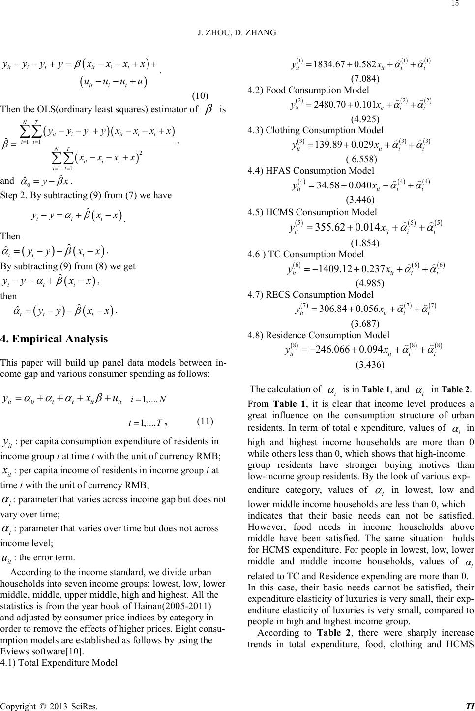

J. ZHOU, D. Z HANG
( )
( )
ititit i t
it i t
yyyyx xxx
u uuu
β − − +=−−++
−−+
.
(10)
Then the OLS(ordinary least squares) estimator of
β
is
()( )
( )
11
2
11
ˆ
NT
ititit i t
it
NT
it i t
it
yy yyxx x x
x xxx
β
= =
= =
−−+ −−+
=
−−+
∑∑
∑∑
,
and
0
ˆ
ˆyx
αβ = −
.
Step 2. By subtracting (9) from (7) we have
( )
ˆ
i ii
yy xx αβ −= +−
,
Then
() ()
ˆ
ˆ
iii
yy xx αβ = −−−
.
By subtracting (9) from (8) we get
( )
ˆ
t tt
yyxx αβ −= +−
,
then
() ()
ˆ
ˆtt t
yy xx αβ = −−−
.
4. Empirical Analysis
This paper will build up panel data models between in-
come gap and various consumer spending as follows:
0itititit
y xu ααα β = ++++
1,...,iN=
1,...,tT=
, (11)
it
y: per capita consumption expenditure of residents in
income group i at time t with the unit of currency RMB;
it
x
: per capita income of residents in income group i at
time t with the unit of currency RMB;
i
α
: parameter that varies across income gap but does not
vary over time;
t
α
: parameter that varies over time but does not across
income level;
it
u
: the error term.
According to the income standard, we divide urban
households into seven income groups: lowest, low, lower
middle, middle, upper middle, high and highest. All the
statistics is from the year book of Hainan(2005-2011)
and adjusted by consumer price indices by category in
order to remove the effects of higher prices. Eight consu-
mption models are established as follows by using the
Eviews software[10].
4.1) Total Expenditure Model
( )( )( )
1 11
1834.67 0.582
itit it
yx αα = + ++

(7.084)
4.2) Food Consumption Model
( )( )( )
2 22
2480.70 0.101
itit it
yx αα =+ ++

(4.925)
4.3) Clothing Consumption Model
( )( )( )
3 33
139.89 0.029
ititit
yx αα = +++

( 6.558)
4.4) HFAS Consumption Model
( )( )( )
4 44
34.58 0.040
itit it
yx αα = +++

(3.446)
4.5) HCMS Consumption Model
( )( )( )
5 55
355.62 0.014
itit it
yx αα = +++

(1.85 4)
4.6 ) TC Consumption Model
( )( )( )
6 66
1409.12 0.237
itit it
yx αα =− +++

(4.985)
4.7) RECS Consumption Model
( )( )( )
7 77
306.84 0.056
itit it
yx αα = +++

(3.68 7)
4.8) Residence Consumption Model
( )( )()
8 88
246.066 0.094
itit it
yx αα =−+++

(3.436)
The calculation of
i
α
is in Table 1, and
t
α
in Table 2.
From Table 1, it is clear that income level produces a
great influence on the consumption structure of urban
residents. In term of total e xpenditure, values of
i
α
in
high and highest income households are more than 0
while others less than 0, which shows that high-income
group residents have stronger buying motives than
low-income group residents. By the look of various exp-
enditure category, values of
i
α
in lowest, low and
lower middle income households are less than 0, which
indicates that their basic needs can not be satisfied.
However, food needs in income households above
middle have been satisfied. The same situation holds
for HCMS expenditure. For people in lowest, low, lower
middle and middle income households, values of
i
α
related to TC and Residence expending are more than 0.
In this case, their basic needs cannot be satisfied, their
expenditure elasticity of luxuries is very small, their exp-
enditure elasticity of luxuries is very small, compared to
people in high and highest income group.
According to Table 2, there were sharply increase
trend s in total expenditure, food, clothing and HCMS
15

J. ZHOU, D. Z HANG
Table 1. Calculation of income level factor
i
α
Income
Gap
Total
Expenditure
Food Clothing HF AS HCMS TC RECS Residence
Lowe st -716.89 -975.76 -118.71 -51.37 -277.06 811.71 -260.09 282.33
Low -574.24 -538.25 -108.17 -66.64 -262.99 530.18 -275.86 219.57
Lower
Midd le
-436.49 -312.48 -78.64 -74.13 -131.52 272.39 -228.57 180.15
Midd le -68.10 123.98 -43.52 -68.36 7.17 53.47 -108.36 10.99
Upper
Midd le
-162.67 311.78 52.26 10.13 18.81 -416.96 30. 86 -162.18
High 8 29.67 702.70 136 .02 27.48 216.67 -653.34 333.22 7.46
Highest 1128.73 688.03 160.79 222.90 428.93 -597.4 4 508.81 -538.33
Table 2. Calculation of time factor
t
α
Year
Total
Expenditure
Food Clothing HF AS HCMS TC RECS Residence
2004 -425.43 -448.51 -27.98 -35.98 -72.99 153.19 16.44 55.68
2005 -593.89 -388.20 -42.24 -48.89 -37.60 21.01 -38.80 -32.45
2006 142.68 -300.15 -19.49 34.51 -61.14 463.64 47.88 5.73
2007 187.96 -294.89 -6.80 84.12 38.28 328.25 21.28 7.13
2008 317.90 96.58 -27.57 7.39 39.65 -190.83 31.00 234.55
2009 565.92 753.84 72.71 8.52 74.45 -317.76 -3.67 1.310
2010 -195.14 581.33 51.38 -49.68 19.34 -457.51 -74.13 -271.95
Table 3. Period to period growth rate of time factor
t
α
Year
Total
Expenditure Food Clothing HFAS HCMS TC RECS Residence
2005
-0.395
0.134
-0.510
-0.359
0.485
-0.863
-3.360
-1.583
2006
1.240
0.227
0.539
1.706
-0.626
21.068
2.234
1.177
2007
0.317 0.0175 0.652 1.438 1.626 -0.292 -0.556 0.244
2008
0.691 1.328 -3.055 -0.912 0.036 -1.581 0.457 31.896
2009
0.780 6.805 3.637 0.153 0.878 -0.665 -1.118 -0.994
2010
-1.344
-0.229
-0.293
-6.831
-0.740
-0.440
-19.199
-208.595
consumption from 2004 to 2009. In 2010, total
expenditure and expenses in each category tend to come
down because of the catastrophic flood damage which is
rarely seen in the history. For instance, values of
t
α
in
HFAS, TC, RECS and Residence are less than 0, which
shows that residents do not dare to spend money in this
period. To analysis the direction of expenses in each
category, we calculate the period to period growth rate of
time factor
t
α
as Table 3. It is very straight-forward
that residence consumption fluctuated remarkably after
2007. Reason is that the building of the International
Tourism Island leads to a house-price boom, which re-
flects the unreasonable economic structure.
5. Conclusion
From the above analysis, we can conclude that urban
residents’ living standards have been improved in Hainan
in recent years. But income factor remains an important
factor that affects urban residents’ consumption structure.
Widening of income gap has significant effects on con-
sumption. Narrowing the income distribution gap is es-
sential for supporting consumption and adjusting con-
sumption structure. The government should hold firmly
the great opportunity of enhancing the building of the
International Tourism Island to the national strategy,
16

J. ZHOU, D. Z HANG
make use of superiority in various respects in Hainan,
widen finance investments, speed up the adjustment of
the economic structure, increase employment and raise
residents' income.
5. Acknowledgements
This work is partially supported by Hainan Provincial
Natural Science Fund (112001), Young Teacher Funded
Research Project of Hainan Normal University (QN1233)
and the Scientific Research Foundation of Yunnan Prov-
ince Education Committee (2011C120).
REFERENCES
[1] A. Blinder, “The Relationship between Distribution Ef-
fects and the Consumption,” The Journal of Political
Economy, Vol. 132, No. 3, 2002, pp. 447-476.
[2] D. Valley, A. Philips, “Studies in Inequality of Income
and Consumption Function: Some Cross-Country Re-
sults,” The Journal of Political Economy, Vol. 133, No. 6,
2003, pp. 132-157.
[3] P. Musgrove, “Income Distribution in countries During
the Period of Economic Reform and Globalization,” The
Journal of Political Economy, Vol. 102, No. 3, 2005, pp.
34-105.
[4] F. Sun, D. H. Yi, “Analysis of Income Distribution Effect
on Chinese Urban Households Consumption Structure,”
Statistical Research, No. 3, 2000, pp. 9-15.
[5] J. Li, “Quantitative Analysis of Income Gap Effects on
Consumption Demand,” Journal of Quantitative & Tech-
nicalEconomics, No. 9, 2003, pp. 5-11.
[6] Y. Zhang, R.. D. Hu, “Analysis of Chinese Residents’
Income Differentials and Consume Demand,” Forecast-
ing, Vol. 22, No. 2, 2003, pp. 3-6.
[7] L. Y. Chen, “Income Distribution and Underconsump-
tion,” Inquiry into Economic Issues, No. 4, 2005, pp.
23-25.
[8] Hainan bureau of statist, “Hainan Statistical Yearbook,”
Chinese Statistics Press, Beijing, 2005-2011.
[9] H. Cheng, “Analysis of Panel Data,” In: H. Cheng, Sim-
ple Regression with Variable Intercepts, Cambridge Uni-
versity Press, New York, 2003, pp. 27-57.
[10] D. H. Yi, “Data Analysis and Eviews Application,” In: D.
H. Yi, Panel Data Model, Chinese Statistics Press, Bei-
jing, 2002, pp. 201-204.
17