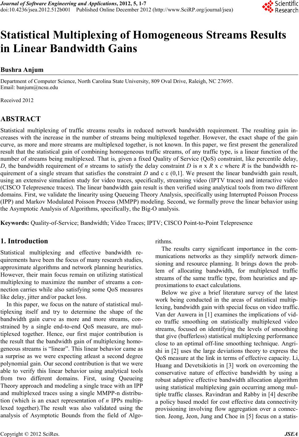Journal of Software Engineering and Applications, 20 12, 5, 1-7
doi:10.4236 /js ea.2012.512b001 Published Online December 2012 (http://www.SciRP.org/journal/jsea)
1
Statistical Multiplexing of Homogeneous Streams Results
in Linear Bandwidth Gains
Bushra Anjum
Department of Compu ter Scien ce, North Carolina St ate University, 809 Oval Drive, R aleigh, NC 27695.
Received 2012
ABSTRACT
Statistical multiplexing of traffic streams results in reduced network bandwidth requirement. The resulting gain in-
creases with the increase in the number of streams being multiplexed together. However, the exact shape of the gain
curve, as more and more streams are multiplexed together, is not known. In this paper, we first present the generalized
result that the statistical gain of combining homogeneous traffic streams, of any traffic type, is a linear function of the
number of streams being multiplexed. That is, given a fixed Quality of Service (QoS) constraint, like percentile delay,
D, the bandwidth requirement of n streams to satisfy the delay constraint D is n x R x c where R is the bandwidth re-
quirement of a single stream that satisfies the constraint D and c ε (0,1]. We present the linear bandwidth gain result,
using an extensive simulation study for video traces, specifically, streaming video (IPTV traces) and interactive video
(CISCO Telepresence traces). The line ar b and width ga in r esult is the n verified usin g analytical tools fro m two differe nt
domains. First, we validate the linearity usin g Queueing T heory Analysis, spec ifically using Inter rupted Po isso n Process
(IPP) and Markov Modulated Poisson Process (MMPP) modeling. Second, we forma lly p ro ve the l ine ar b eha vior usin g
the Asymptotic Analysis of Algorithms, specifically, t he Big-O analysis.
Keywords: Quality-of-Service; Bandwid th; Video Traces; IPTV ; CISCO Point-to -Point Telepresence
1. Introduction
Statistical multiplexing and effective bandwidth re-
quirements have been the focus of many research studies,
approximate algorithms and network planning heuristics.
However, their main focus remain on utilizing statistical
multiplexing to maximize the number of streams a con-
nection carries while also satisfying some QoS measures
like delay, jitter and/or pa c ket loss.
In this paper , we foc us on the nature of statistica l mul-
tiplexing itself and try to determine the shape of the
bandwidth gain curve as more and more streams, con-
strained by a single end-to-end QoS measure, are mul-
tiplexed together. Hence, our first major contribution is
the result tha t the bandwidth gain of multiplexing ho mo-
geneous streams is “linear”. This linear behavior came as
a surprise as we were expecting atleast a second degree
pol yno mia l ga i n. Our se co nd co ntr ib uti o n i s tha t we wer e
able to verify this linear behavior using analytical tools
from two different domains. First, using Queueing
Theory approach and modeling a single trace with an IPP
and multiplexed traces using a single MMPP-n distribu-
tion (which is an exact representation of n IPPs multip-
lexed together).The result was also validated using the
analysis of Asymptotic Bounds from the field of Algo-
rithms.
The results carry significant importance in the com-
munications networks as they simplify network dimen-
sioning and resource planning. It brings down the prob-
lem of allocating bandwidth, for multiplexed traffic
streams of the same traffic type, from heuristics and ap-
proxi mations to e xact c a lculatio ns.
Below we give a brief literature survey of the latest
work being conducted in the areas of statistical multip-
lexing, bandwidth gai n with spe cial fo cus on vid eo traffic.
Van der Auwera in [1] examines the implications of vid-
eo traffic smoothing on statistically multiplexed video
streams, focused on identifying the levels of smoothing
that give (b ufferle ss) sta tistica l multiple xi ng perfor mance
close to an optimal off-line smoothing technique. Angr i-
shi in [2] uses the large deviations theory to express the
Qo S me a s ur e at the link in terms of effective capacity. Li,
Huang and Devetsikiotis in [3] work on overcoming the
conservative nature of effective bandwidth by using a
robust adaptive effective bandwidth allocation algorithm
using statistical multiplexing gain occurring a mong mul-
tiple traffic classes. Ravindran and Rabby in [4] describe
a policy based model for cost effective data connectivity
provisioning involving flow aggregation over a connec-
tion. Jeong, J eon, Jung a nd Choe i n [5] foc us on a statis-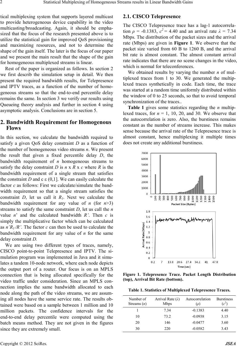

Statistical Multiplexing of Homogeneous Streams results in Linear Bandwidth Gains
Copyright © 20 12 SciRes . JSEA
2
tical multiplexing system that supports layered multicast
to provide heterogeneous device capability in the video
multicasting/broadcasting. Again, it should be empha-
sized that the focus of the research presented above is to
utilize the stat istical gain for improved Q oS provisioning
and maximizing resources, and not to determine the
shape of the gain itself. The later is the focus of our paper
and we present the main result that the shape of the gain
for homogeneous multiplexed streams is linear.
Rest of the paper is organized as follows. In section 2
we first describ the simulation setup in detail. We then
present the required bandwidth results, for Telepresence
and IPTV traces, as a function of the number of homo-
geneous streams so that the end-to-end percentile delay
remains the same. In section 3 we verify our results using
Queueing theory analysis and further in section 4 using
asymptotic analysis. Conclusions are in section 5.
2. Bandwidth Requirement for Homogenous
Flows
In this section, we calculate the bandwidth required to
satisfy a given QoS delay constraint D as a function of
the number of homogeneous video streams n. We present
the result that given a fixed percentile delay D, the
bandwidth requirement of n homogeneous streams to
satisfy the delay constraint D is n x R x c where R is the
bandwidth requirement of a single stream that satisfies
the co nstr a i nt D and c ε (0,1]. We can easily calculate the
factor c as follows: First we calculate/simulate the band-
width requirement so that a single stream satisfies the
constraint D, let us call it R1. Next we calculate the
bandwidth requirement for any value of n (for n>3)
streams to satisfy the same constraint D, let us call the n
value n’ and the calculated bandwidth R’. Then c is
simply the multiplicative factor which can be calculated
as n’R1 /R’. T he factor c can then be used to calculate the
bandwidth requirement for any value of n for the same
delay constraint D.
We are using two different types of traces, namely,
CISCO point-to -point Telepresence and IPTV. The si-
mulation program was implemented in Java and it simu-
lates a tandem 10-node network, where each node depicts
the output port of a router. Our focus is on an MPLS
connection that is being allocated specifically for the
video traffic under consideration. Since an MPLS con-
nection implies the same bandwidth allocated to each
node along the path of the video streams, we are assum-
ing all nodes have the same service rate. The results ob-
tained were based on a sample between 1 million and 10
million packets. The confidence intervals for the
end-to -end delay percentile were computed using the
batch means method. They are not given in the figures
since they are extremely small.
2.1. CISCO Telepresence
The CISCO Telepresence trace has a lag-1 autocorrela-
tion ρ = -0.1383, c2 = 4.40 and an arrival rate λ = 7.34
Mbps. The distribution of the packet sizes and the arrival
rate (Mbps) are given in Figure 1. We observe that the
packet size varied from 60 B to 1260 B, and the arrival
bit rate is almost constant. The almost constant arrival
rate indicates that there are no scene changes in the video,
which is normal for teleconferences.
We obtained results by varying the number n of mul-
tiplexed traces from 1 to 30. We generated the multip-
lexed traces synthetically in code. Each time, the trace
was started at a random time uniformly distributed within
the window of 0 to 25 seconds, so that to avoid temporal
synchronization of the traces..
Table 1 gives some statistics regarding the n multip-
lexed traces, for n = 1, 10, 20, and 30. We observe that
the autocorrelation is zero. Also, the burstiness remains
constant as the number of streams increase. This makes
sense because the arrival rate of the Telepresence trace is
almost constant, hence multiplexing it multiple times
does not create any additional burstiness.
Figure 1. Telepresence Trace. Packet Length Distribution
(top), Arrival Bit Rate (bottom).
Table 1. Statistics of Multiplexed Telepresence T races.
Number of
Strea ms (n) Arrival Rate (λ) Mbps Aut ocorrelation (ρ) Bu r st iness (c2)
1 7.34 -0.138 3 4.40
10 73.2 -0. 0938 3.15
20 146 -0.047 7 3.60
30 220 -0.058 2 3.43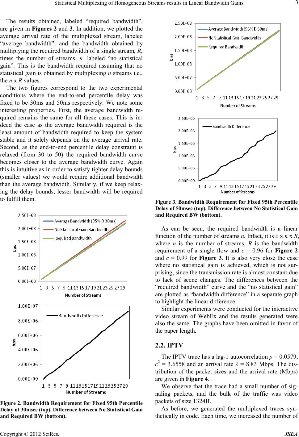

Statistical Multiplexing of Homogeneous Streams results in Linear Bandwidth Gains
3
The results obtained, labeled “required bandwidth”,
are given in Figures 2 and 3. In addition, we plotted the
average arrival rate of the multiplexed stream, labeled
“average bandwidth”, and the bandwidth obtained by
multiplying the required bandwidth of a single stream, R,
times the number of streams, n. labeled “no statistical
gain”. This is the bandwidth required assuming that no
statistical gain is ob tained by multiplexing n str eams i.e.,
the n x R values.
The two figures correspond to the two experimental
conditions where the end-to -end percentile delay was
fixed to be 30ms and 50ms respectively. We note some
interesting properties. First, the average bandwidth re-
quired remains the same for all these cases. This is in-
deed the case as the average bandwidth required is the
least amount of bandwidth required to keep the system
stable and it solely depends on the average arrival rate.
Second, as the end-to-end percentile delay constraint is
relaxed (from 30 to 50) the required bandwidth curve
becomes closer to the average bandwidth curve. Again
this i s int uitive a s in or der t o satis fy tighte r del ay bo unds
(smaller values) we would require additional bandwidth
than the average bandwidth. Similarly, if we keep relax-
ing the delay bounds, lesser bandwidth will be required
to fulfill them.
Figure 2. Bandwidth Require ment for Fix ed 95th Percentile
Delay of 30msec (top). Di f feren ce between No Stati s t ical Gain
and Requi red BW (bottom).
Figure 3. Bandw i dth Req uire ment for Fi x ed 95 th Per centile
Delay of 50msec (to p). Difference between No Statistic al Gain
and Requi red BW (bottom).
As can be seen, the required bandwidth is a linear
function of the number of streams n. Infact, it is c x n x R,
where n is the number of streams, R is the bandwidth
requirement of a single flow and c = 0.96 for Figure 2
and c = 0.99 for Figure 3. It is also very close the case
where no statistical gain is achieved, which is not sur-
prising, since t he tra ns mission rate is almost consta nt d ue
to lack of scene changes. The differences between the
“required bandwidth” curve and the “no statistical gain”
are plotted as “bandwidth difference” in a separate graph
to highlight the li nea r difference.
Similar experiments were conducted for the interactive
video stream of WebEx and the results generated were
also the same. The graphs have been omitted in favor of
the paper length.
2.2. IPT V
The IPTV trace has a lag-1 autocorrelation ρ = 0.0579,
c2 = 3.6558 and an arrival rate λ = 8.83 Mbps. The dis-
tribution of the packet sizes and the arrival rate (Mbps)
are gi ven in Figure 4.
We observe that the trace had a small number of sig-
naling packets, and the bulk of the traffic was video
packets of size 1324B.
As before, we generated the multiplexed traces syn-
thetically in code. Each time, we increased the number of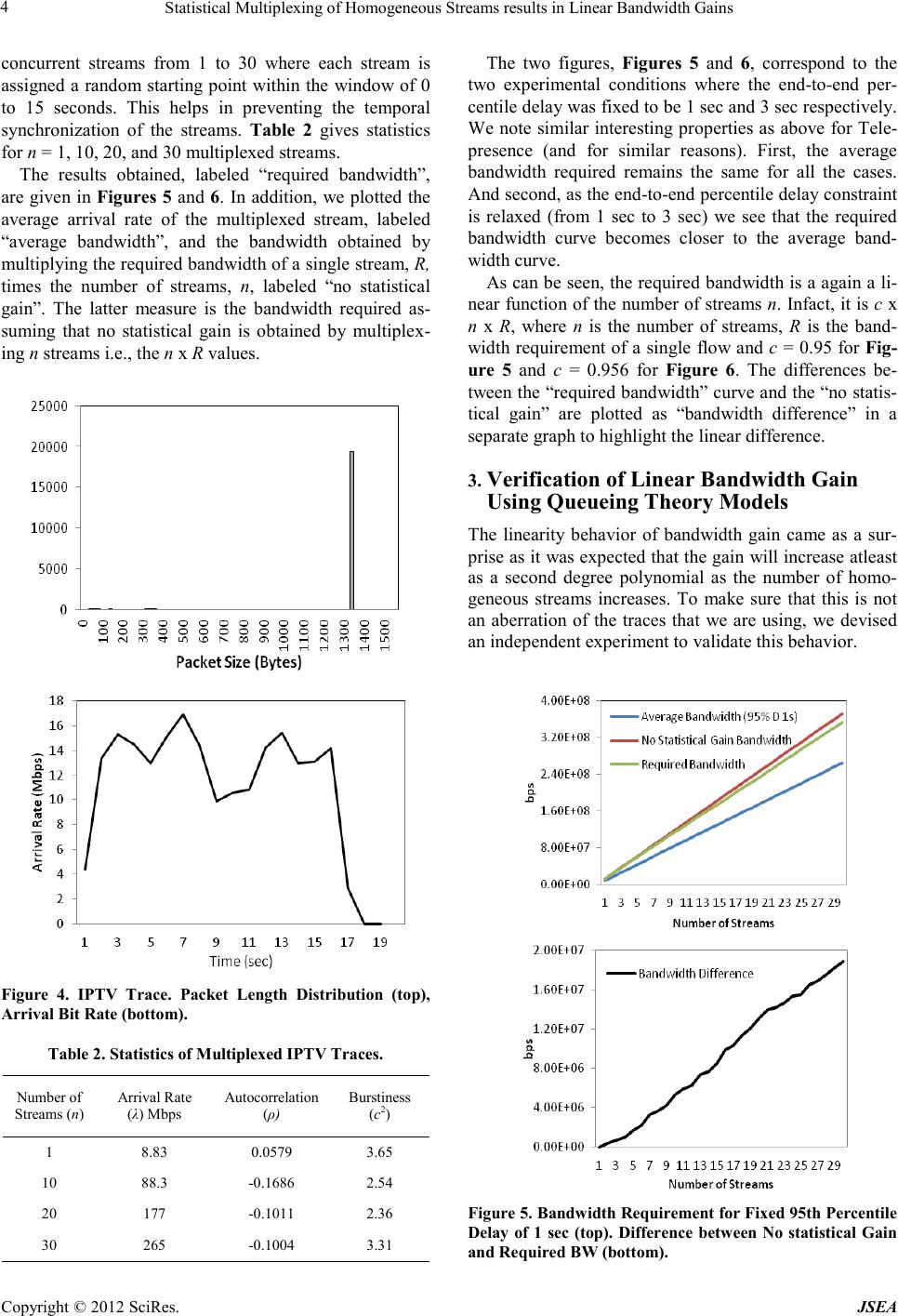

Statistical Multiplexing of Homogeneous Streams results in Linear Bandwidth Gains
Copyright © 20 12 SciRes . JSEA
4
concurrent streams from 1 to 30 where each stream is
assigned a random starting point withi n the window of 0
to 15 seconds. This helps in preventing the temporal
synchronization of the streams. Table 2 gives statistics
for n = 1, 10, 20, and 30 multiplexed streams.
The results obtained, labeled “required bandwidth”,
are given in Figures 5 and 6. In addition, we plotted the
average arrival rate of the multiplexed stream, labeled
“average bandwidth”, and the bandwidth obtained by
multiplying the required bandwidth of a single stream, R,
times the number of streams, n, labeled “no statistical
gain”. The latter measure is the bandwidth required as-
suming that no statistical gain is obtained by multiplex-
ing n streams i.e., the n x R values.
Figure 4. IPTV Trace. Packet Length Distribution (top),
Arrival Bit Rate (bottom).
Table 2. Statistics of Multiplexed IPTV Traces.
Number of
Streams ( n) Arrival Rate (λ) Mbps Autocorrelation (ρ) Bu rstiness (c2)
1 8.83 0.0579 3.65
10 88.3 -0. 1686 2.54
20 177 -0.101 1 2.36
30 265 -0.100 4 3.31
The two figures, Figures 5 and 6, correspond to the
two experimental conditions where the end-to-end per-
centile delay was fixed to be 1 sec and 3 sec respectively.
We note similar interesting properties as above for Tele-
presence (and for similar reasons). First, the average
bandwidth required remains the same for all the cases.
And se cond , as the e nd-to -end per centile delay constraint
is relaxed (from 1 sec to 3 sec) we see that the required
bandwidth curve becomes closer to the average band-
width curve.
As can be seen, the required bandwidth is a again a li-
near function of the number of streams n. Infact, it is c x
n x R, where n is the number of streams, R is the band-
width requirement of a single flow and c = 0.95 for Fig-
ure 5 and c = 0.956 for Figure 6. The differences be-
twee n the “requir ed ba ndwid th” c urve a nd the “no st atis-
tical gain” are plotted as “bandwidth difference” in a
separate graph to highlight t he linear difference.
3. Verification of Linear Bandwidth Gain
Using Queueing Theory Models
The linearity behavior of bandwidth gain came as a sur-
prise as it was expected that the gain will increase atleast
as a second degree polynomial as the number of homo-
geneous streams increases. To make sure that this is not
an aberration of the traces that we are using, we devised
an independent expe rime nt to validate this behavior.
Figure 5. Bandw idt h Req uire ment f or Fi xe d 95t h Perce ntile
Delay of 1 sec (top). Difference between No statistical Gain
and Requi red BW (bottom).

Statistical Multiplexing of Homogeneous Streams results in Linear Bandwidth Gains
5
An Interrupted Poisson Process (IPP) modulates be-
tween two exponentially distributed states, an ON and an
OFF state. T he tra nsition rate s for the ON a nd OFF sta tes
are respectively α and β, see Figure 7. While in the ON
state, the process generates Poisson arrivals with rate λ
whereas in the OFF state there are no arrivals.
The aggregate of n homogeneous IPPs (with parame-
ters α, β and λ) is the well known Markov Modulated
Poi sson Process (MMPP) with n+1 states. This a ggregate
process of n homogenous IPPs i s given in Figure 8.
Figure 6. Bandw i dth Req uire ment for Fi x ed 95 th Per centile
Delay of 3 sec (top). Difference between No statistical Gain
and Requi red BW (bottom)
Figure 7. M arkov Chain of an IPP.
Figure 1. Markov Chain of an (n+1) state MMPP,
representi ng n aggregate homogeneous IPPs
An IPP effectively models a VoIP call characteristics,
i.e. , voi ce sp urts a nd s ilent per iods. So, we ca n use an IPP
to represent one VoIP call, or in other words, one stream.
Next, we want to multiplex similar VoIP calls together.
This will effectively mean multiplexing the same IPP
multiple times. It is a well known result in Queueing
theory that multiplexing n IPPs results in the n-state
MMPP process. Hence we use the resultant MMPP to
represent multiplexed IPP streams.
The parameter values chosen for the IPP stream are set
equal to the parameter values of a VoIP call. A VoIP has,
on average, 400 ms of ON period, 600 ms of OFF period
[6], and the number of packets generated per second
during the ON period is 50. A voice payload of 160 bytes
is carried in a separate IP packet with a 40-byte IP/
UDP/RTP header. Thus, we have α = 2.5, β = 1.667 and
λ = 50. The QoS constraint enforced is that the 95th per-
centile delay should be less than equal to 50 msec.
As can be seen in Figure 9, once again the required
bandwidth is a linear function of the number of streams n.
Infact, it is c x n x R, where n is the number of streams, R
is the bandwidth requirement of a single flow and c =
0.06. The differences between the “required bandwidth”
curve and the “no statistical gain” are plotted as “band-
width difference” to highlight the linear difference between
curves. Interestingly, we see a huge gain in bandwidth
Figure 9. Bandw idt h Req uire ment f or Fi xe d 95t h Perce ntile
Delay of 50 msec (top). Difference between No statistical
Gain and Required BW (bottom)

Statistical Multiplexing of Homogeneous Streams results in Linear Bandwidth Gains
Copyright © 20 12 SciRes . JSEA
6
here. The bandwidth gain increases as burstiness of orig-
inal traffic increases and as arrival rate of the original
traffic decreases, but, it retains its linear characteristic.
An IPP is highly bursty because the arrivals are batched
toget her duri ng the ON p eriod and no ar rivals oc cur dur-
ing the OFF peri od.
We would like to mention here that the linear ity beha-
vior has been indepe ndently confirmed by Lone [7].
4. Validation of Linear Bandwidth Gain
Using Algorithmic Asymptotic Analysis
The linear behavior can also be explained by the algo-
rithmic a symptotic analys is. For thi s, we will use the def i-
nition of big-theta Θ which implies as ymptotic “equa lit y”.
Before we proceed we need to define big-oh O and
big-omega Ω. The following definitions and Figure 10
are taken from [8].
Definition o f big-oh: Let f and g b e functio ns fro m the
set of integers (or the set of real numbers) to the set of
real numbers. Then f(n) is said to be O(g(n)) , if and onl y
if there are constants C and n0 such that
| f(n)| ≥ C |g(n)| , whenever n > n0
Big-oh is concerned with the "less than or equal to"
relation between functions for large values of the varia-
ble. It is also possible to consider the “greater than or
equal to” relation (big-Omega) and “equal to” relation
(big-theta) in a similar wa y.
Definition of big-omega: f(n) is said to be Ω(g(n)), if
there are constants C and n0 such that
|f(n)| ≤ C |g(n) | , whenever n > n0
Definition o f big-theta: f(n) is said to be Θ(g(n)), if f(n)
is O(g(n)) and f(n) is Ω(g(n)). We also say that f(n) is of
order g(n) or that both f and g are of the same order.
f(n)= Θ(g(n)) implies: f(n) “=”g(n). Formally, Θ(g(n)) =
{f(n) : there exist positive constants c1, c2 and n0 such
that, 0 ≤ c1g(n) ≤ f(n) ≤ c2 g(n) for all n ≥ n0}.
This is repr e sented pictorially in Figure 10, i.e., g(n) is
an asymptotically tight bound for f(n).
Figure 10. Pictorial R epresentation of big-theta.
In all four figures (Figures 2-5), the required band-
width curve is bounded by the average bandwidth curve
from below and the no statistical gain curve from above.
The average bandwidth curve is linear, since the average
bandwidth of n strea ms is n times the average bandwidth
of a single stream. Similarly the no statistical gain (or
maximum bandwidth) curve is linear and for the same
reason.
Let us name the required bandwidth curve as f(n),
where n is the number of streams, and let us define a
function g(n) = n. We can define the average bandwidth
curve by the straight line g1(n) = m1n, where m1 is the
average bandwidth required for a single stream. Similarly,
the no statistical gain curve can be defined by the straight
line g2(n) = m2n, where m2 is the bandwidth required for
a single stream. Now we have all the components of the
big-theta definition, i.e.,
0 ≤ g1(n) ≤ f(n) ≤ g2(n) for all n ≥ 0 or
0 ≤ m1n ≤ f(n) ≤ m2n for all n ≥ 0 or
0 ≤ m1g(n) ≤ f(n) ≤ m2 g(n) for a ll n ≥ 0
Hence by definition of big-theta, f(n) = Θ(g(n)) or f(n)
“=”g(n). As g(n) is a linear function, hence f(n) will also
be a linear function.
Thus we ded uce tha t i f a func t ion f(n) is bounded from
above by a linear function and also from the below by a
linea r function, the n it also behaves in a linear fashion.
5. Conclusion
In this paper, we first presented the generalized result
that the statistical gain of combining homogeneous traffic
streams, of any traffic type, is a linear function of the
number of streams being multiplexed, for a fixed QoS
constraint like percentile delay. We then presented linear
bandwidth gain results for actual video traces, streaming
video (IPTV traces) and interactive video (CISCO Tele-
presence traces). The linear bandwidth gain result is fur-
ther verified using IPP and MMPP modeling and Big-O
asymptotic analysis.
REFERENCES
[1] G. Van der Auwera, "Implications of Smoothing on Sta-
tistical Multiplexing of H.264/AVC and SVC Video
Streams," IEEE Transactions on Broadcasting, vol. 55, no.
3, pp. 541-558, Sep. 2009.
[2] K. Angrishi, "Analysis of a Real-Time Network using
Statistical Network Calculus with Effective Bandwidth
and Effective Capacity," in 14th GI/ITG Conference on
Measuring, Modeling and Evaluation, 2008, pp. 1-15.
[3] H. Li, C. Huang, and M. Devetsikiotis, “A Robust Adap-
tive Effective Bandwidth Allocation Technique,” in IEEE
International Conference on Communications, 2005, pp.
115-119.
[4] K. Ravindran, M. Rabby, and X. Liu, "Bandwidth mea-
surement and management for end-to-end connectivity

Statistical Multiplexing of Homogeneous Streams results in Linear Bandwidth Gains
7
over IP networks," in First International Communication
Systems and Networks and Workshops, 2009, pp. 1-8.
[5] J. Jeong, S. Jeon, Y. H. Jung, and Y. Choe, "Statistical
Multiplexing using scalable video coding for layered
multicast," in IEEE International Symposium on Broad-
band Mul ti me dia Sy s tems , 2009, pp. 1-5.
[6] H. G. Perros, Connection-Oriented Networks: SONET/
SDH, ATM, MPLS, and OPTICAL NETWORKS, Wiley,
2005.
[7] Q. B. Lone, "Bandwidth Allocation for Video Streams
Subject To An End-to-End P ercentile Del ay," MS Th esis,
North Carolina State University, 2011.
[8] T. H. Cormen, C. E. Leiserson, R. L. Rivest, and C. Stein,
Introduction to Algorithms, 3rd ed. Massachusetts Insti-
tute of Technology, 2009.