Multicut L-Shaped Algorithm for Stochastic Convex
Programming withFuzzy Probability Distribution
Miaomiao Han
School of Mathematics and Physics
North China Electric Power University
Baoding, Hebei Province, China
Xinshun MA
School of Mathematics and Physics
North China Electric Power University
Baoding, Hebei Province, China
Abstract—Two-stage problem of stochastic convex programming with fuzzy probability distribution is studied in this
paper. Multicut L-shaped algorithm is proposed to solve the problem based on the fuzzy cutting and the minimax rule.
Theorem of the convergence for the algorithm is proved. Finally, a numerical example about two-stage convex recourse
problem shows the essential character and the efficiency.
Keywords-stochastic convex programming;fuzzy probability distribution; two-stage problem; multicut L-shaped
algorithm
1. Introduction
Stochastic programming is an important class of
mathematical programming with random parameters, and
has been widely applied to various fields such as economic
management and optimization control[1]. Two-stage
stochastic programming is a kind of mathematical
programming where the decision variables and the decision
process can be decomposed into two stages based on
random parameters are observed before and after the
specific value.
Stochastic linear programming as a basic issue has been
studied widely, and many research results have been
reported.In [2], two-stage problem of stochastic linear
programming and the basic algorithm were first proposed
and applied to the linear optimal control problem. Since
then, a large variety of algorithms including Benders
decomposition[2][3], stochastic decomposition[4], subgradient
decomposition[5][6], nested decomposition[7], and disjunctive
decomposition[8] for the two-stage stochastic linear
programming had been developed. Among these methods,
Benders decomposition also called the L-shaped method
has become the main approach to deal with stochastic
programming problems.
The theories and algorithmsobtained before on
stochastic linear programming all arebased on a hypothesis
that the probability distributions of random parameters have
completely information. However, in many situations, due
to lack of the date, the probability of a random event is not
fully known, and need to get an approximate range with the
help of experts’ experience. Recently, model of the
stochastic linear program with fuzzy probability distribution
was proposed in [9], and the modified L-shaped algorithm
was presented to solve the model.
Stochastic convex programming is an important class of
stochastic nonlinear program and has more widely
application than stochastic linear programming[10].As a
result, stochastic convex programming with fuzzy
probability distribution will havemore useful in many
practical situations. In this paper, two-stage stochastic
convex programming with fuzzy probability distribution
and the solving method are studied, a numerical example
shows the essential character and the efficiency.
2. Two-stage stochastic convex
programming under fuzzy probability
distribution
Let

,,P:¦ be a probability space, sample space
^`
1
,,
N
ZZ : "
is a finite set, and
¦
=
2
:
is the
V
-algebra
composed by power set of :
,
^`
.
ii
pP ZZ
The two-
stage stochastic convex programming problem is
1
()(,)
. .
0
N
ii
i
minfxp Qx
st Ax b
x
Z 
t
¦
(1)
whereˈ
(,) (,)
. . ()()
0
ii
ii
Qx mingy
st WyhTx
y
ZZ
ZZ 
t
(2)
1
n
x
and
2
n
y
are decision vectors,
()fx
is convex
function, Ais
11
mnu matrix,
1
m
b is known vector,
W
is
22
mnu
recourse matrix, for each i
Z :,(, )
i
gy Z
is
convex function on y ,
2
()
m
i
h Z  is vector, and

i
T Z is
Open Journal of Applied Sciences
Supplement：2012 world Congress on Engineering and Technology
Cop
y
ri
g
ht © 2012 SciRes.219

21
mnumatrix. Where
x
and
y
are the first stage decision
variable and the second stage decision variable respectively.
The mathematical expected value
1
[(,)](,)
N
ii
i
EQx pQx ZZ
¦
.
When the random variable obeys fuzzy probability
distribution, the scope of i pis as follows[9]
  ^
`
1
|11 ,
1;0,1,,
N
iiiiiii
N
ii
i
Pd lpd l
ppi N
D
SDD dd
t
¦
"
(3)
where

12
,,,
TN
N
Ppp p " consisted of probabilities,

1
,,
T
N
ll l "
denotes the vagueness level, and the level
value (0 1)
i
DD dd expresses the DM credibility degree of
the partial information on probability distribution. Thefuzzy
probability distributions results in that mathematical
expectation [(,)]EQx Z
is uncertain, here,
[(,)]
p
P
max EQx
D
S
Z

=
1
(,)
N
ii
Pi
maxp Qx
D
S
Z

¦
will be used to instead of
[(,)]EQx Z
, and
then (1) can be expressed as follows
1
()(,)
. .
0
N
ii
Pi
minfxmaxpQx
st Ax b
x
D
S
Z


t
¦
(4)
where (, )
i
Qx Z is confirmed by(2).
Obviously, for a given x
, there
exists
12
(, ,,)
T
N
Ppp p "
D
S , such that
11
(, )(, )
NN
ii ii
P
ii
pQ xmaxpQ x
D
S
ZZ

¦¦
.
I. MULTICUT L-SHAPED ALGORITHM
The problem(4) is equivalent to:
1
12
(),
.. (,),
,
x
N
ii
Pi
min f x
s tmaxp Qx
xK KK
D
S
T
ZT


d

¦

(5)
where
(, ) (,),
. . ()(),
0,
i
iii
y
ii i
i
Qx min gy
st WyhTx
y
Z Z
ZZ 
t
(6)
and
`
^
1,0,KxAxbx t
`
^
2
, 0,.. ()().
ii iii
Kxforallys tWyhTx ZZZ :t 
The standard L-shaped algorithm for solving above
problem can be designed under outer linearization (see e.g.
[9]). Suppose that
12
(, ,,)
T
N
Ppp p "
is solution of
1
(,)
N
ii
Pi
maxp Qx
D
S
Z

¦
, problem (5) can be replaced by the
following (7)
1
12
(, )
()
.. ,
i
N
ii
xi
i
Qx
min f xp
s tforalli
xK KK
Z
T
T

d

¦

(7)
because of each constrain in (5) corresponds to
Nconstraints in (7).
The multicut L-shaped algorithm is defined as follows:
S0. Set 0,sk 0
i
t for all
1, 2,,iN "
, and
0
x is
given.
S1. Set 1kk 
, solve the following master problem:
1
() ()
()(a1)
.. ,0,(a2)
,1,2,,, (a3)
,()1,2,,, (a4)
1, 2,,
N
ii
i
ll
lii lii
min fxp
stAxb x
Dx dls
Exe lit
iN
T
T

°
° t
°
®t
°
°t
°
¯
¦
"
"
"
(8)
Let

1
,,,
kk k
N
x TT " be an optimal solution of
problem(8). Note that if no constraint (a4)
is presentfor
some i ,
k
i
T is set equal to f ,
k
i
T and i parenot
considered in the calculation of
k
x . Go to S2.
S2. For 1, ,iN ", solve the following linear
programming problems
. . ()() (a5)
0,0,0
TT
i
k
ii
min zeueu
s tWyIuIuhTx
yu u
ZZ



 
° 
®
°ttt
¯
(9)
where

1, ,1
T
e " , until, for some i , if the optimal
value 0
i
z!, let
k
V be optimal dual variables value, and
define
1
1
()()
()()
kT
si
kT
si
DT
dh
VZ
VZ



°
®
°
¯
,
set 1ss  , add the constraint
11
k
ss
Dx d

t
to the set
(a3) and return to S1. If for all ,0
i
iz , then go to S3.
S3.For 1, ,iN "
, anda fixed
k
x
, solve the
following convex programming problems
(,)
. . ()() (a6
0 (a7)
ii
k
ii i
i
min g y
st WyhTx
y
Z
ZZ

° 
®
°t
¯
(10)
220 Cop
y
ri
g
ht © 2012 SciRes.

Let (,)
i
k
Qx Z be the optimal value, and
k
i
y the optimal
solution. Solve the problem
1
(,)
N
i
Pi
kk
i
maxp Q x
D
S
Z

¦
, and
suppose
12
(,,,)
kk kT
N
pp p"
is the optimal solution, then
update the objectivefunction of the master problem.
Let
k
i
v and
k
i
u be the optimal dual variables associated
withconstrain (a6) and (a7) respectively. Compute
1
1
() (),
(,)()() [()()].
i
i
kT
tii
kT kkTk
tiiiiiii
EvT
egy uyvWyh
Z
ZZ


 
°
® 
°
¯
If
11
ii
kk
it t
eEx T

 does not hold for any 1, ,iN " ,
stop, then
1
(, ,,)
kk k
N
x TT "
is an optimal solution.
Otherwise, set 1
ii
tt  , add the constraint
11
ii
kk
it t
eEx T

t
to the set
(a4)
, return to S1.
3. Theorem of convergence for the
algorithm
Proposition1. In the algorithm, constraint set(a3) is
finite.
Proof The proof of this proposition is the same to the
standard L-shaped algorithm (see e.g. [2]).
Proposition 2. For any
i
Z :
and on all
i
xK
Z
 ,
(, )
i
Qx Z
is either a finite convex function or is
identically f
,
where ^
`
, 0,.. ()()
iii iii
Kx ystWyh Tx
Z
ZZZ :t  .
Proof (see e.g. [10])
Proposition3. If (, )
i
Qx Z
is a finite convex function
for each
i
Z : , then the function
11
ii
tt
eEx

 islinear
supporting hyper planes of(, )
i
Qx Z .
Proof By the duality theory (see e.g. [11]), it holds
that
(,( , )()()[( )()()] )
kTT k
ii ii
kkkkk
iiiii
Qxgyuy vWy hT x ZZ ZZ  .
We know from the convexity of (, )
i
Qx Z that
(, )(, )( )()[()()]
()().
TT
ii i
T
i
kkkkk
iiiii
k
i
Qxgyuy vWy h
vT x
ZZ Z
Z
t 

Thus
(,)()()[()()]
TT
ii
kkkkk
iiiii
gyuy vWy h ZZ   () ()
T
i
k
i
vT x Z 
11
ii
tt
eEx


is a linear support of (, )
i
Qx Z
.
Theorem. Suppose that the algorithm generates an
infinite sequence of
1
(, ,,)
kk k
N
x TT "
. If
1
(, ,,)
N
x TT "
is the
limit point of an arbitrary subsequence
1
(, ,, )
jj j
kk k
N
x TT "
, and
for each ,i
11
lim() 0
jj
ii
kk
tt i
j
eEx T

of

, 1,, ,iN " then
1
(, ,,)
N
x TT "
is an optimal solution of problem(7), x is an
optimal solution of problem(4).
Proof Since the number of the constraints of
type (a3)
is finite, we have that
j
k
xK
for
j
k
sufficiently
large. We also know K is closed convex set,
then xK
.By known, for each
,i
11
(,)
jj j
ii
kk k
iitt
QxeEx TZ

t 
,
and
11
lim() 0
jj
ii
kk
tt i
j
eEx T

of

Then
(, )
ii
Qx TZ
for all 1, ,iN "
. Thus,
1
(, ,,)
N
x TT "
is a feasible solution
of problem(7).
On the other hand, if
x

is optimal solution to the
minimax problem(4), but not necessarily an optimal solution
in iteration
j
k
, then
*
11
() (,)() (,).
jj
NN
kk
ii ii
PP
ii
fxmaxp Qxfxmaxp Qx
DD
SS
ZZ


d
¦¦
By continuity of the convex function we have that
*
11
()(, )()(, )
NN
iii i
PP
ii
fxmaxp Qxfxmaxp Qx
DD
SS
ZZ


d
¦¦
,
then, for a certain value
12
(, ,,)
T
N
pp p
D
S "
*
11
()( )( ,),
NN
iiii
P
ii
fxpfxmax pQx
D
S
TZ


d
¦¦
Hence,
1
(, ,,)
N
x TT " is an optimal solution to problem(7),
and xis an optimal solution to problem(4).
4. Numerical example
Consider the following two-stage stochastic convex
programming
12
22
12
12 12
12 11
122 2
112 2
1212
3
3.552
22
. . 25, ,
3, 2,
,,,
,
0.
,
x
min xx
yy
Eminyyyy
stx xyx
xxyx
x
y
yy
y
[
[[


°½
°
°
®¾
°°¿
¯
°
°
®t d
°d d
°
°d
¯t
d
°
°
(11)
where
1
[
takes the three values 3.5, 3.8 and 4.0 with
probability 1/3, that2 [ takes the values 0.5, 1.0and 1.5 with
probability 1/3, and that
1
[ and 2 [ are independent of each
other, then
12
(,)
T
[[[ can take the each vector in the set
12
{(,)|
T
kk3
12
3.5,3.8,4.0,0.5,1.0,1.5}kk with probability 1/9.
Under fuzzy probabilitydistribution, assume that [
takes the each values in
3
with probability around 1/9, i.e.
i
p#1/9 (1,2,,9)i "ˈit can be confirmed by(3),
where 1/12
i
d ,
Cop
y
ri
g
ht © 2012 SciRes.221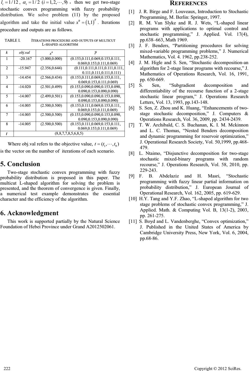

1/12
i
l , 1/2
i
D
(1,2,,9)i "ˈthen we get two-stage
stochastic convex programming with fuzzy probability
distribution. We solve problem (11) by the proposed
algorithm and take the initial value

0
1,1
T
x
.Iterations
procedure and outputs are as follows.
TABLE I. ITERATIONS PROCEDURE AND OUTPUTS OF MULTICUT
L-SHAPED ALGORITHM
k .obj val
k
x
P
1-20.167(3.000,0.000)(0.153,0.111,0.069,0.153,0.111,
0.069,0.153,0.111,0.069)
2-15.947 (2.356,0.644)(0.111,0.111,0.111,0.111,0.111,
0. 111,0.111 ,0. 11 1,0.111)
3-14.454(2.566,0.434) (0.153,0.111,0.069,0.153,0.111,
0.069,0.153,0.111,0.069)
4-14.020(2.501,0.499) (0.153,0.090,0.090,0.153,0.090,
0.090,0.153,0.090,0.090)
5-14.007(2.499,0.501) (0.153,0.090,0.090,0.153,0.090,
0.090,0.153,0.090,0.090)
6-14.005(2.500,0.500) (0.153,0.111,0.069,0.153,0.111,
0.069,0.153,0.111,0.069)
7-14.005(2.500,0.500) (0.153,0.090,0.090,0.153,0.090,
0.090,0.153,0.090,0.090)
8-14.005(2.500,0.500) (0.153,0.111,0.069,0.153,0.111,
0.069,0.153,0.111,0.069)
t
(8,8,7,7,8,5,6,8,5)
Where obj.val refers to the objective value,
19
(,, )tt t "
is the vector on the number of iterations of each scenario.
5. Conclusion
Two-stage stochastic convex programming with fuzzy
probability distribution is proposed in this paper. The
multicut L-shaped algorithm for solving the problem is
presented, and the theorem of convergence is given. Finally,
a numerical test example demonstrates the essential
character and the efficiency of the algorithm.
6. Acknowledgment
This work is supported partially by the Natural Science
Foundation of Hebei Province under Grand A2012502061.
REFERENCES
[1]J. R. Birge and F. Louveaux, Introduction to Stochastic
Programming, M. Berlin: Springer, 1997.
[2]R. M. Van Slyke and R. J. Wets, “L-shaped linear
programs with applications to optimal control and
stochastic programming,” J. Applied. Vol. 17(4),
pp.638–663, Math1969.
[3]J. F. Benders, “Partitioning procedures for solving
mixed-variable programming problems,” J. Numerical
Mathematics, Vol. 4. 1962, pp.238-252.
[4]J. M. Higle and S. Sen, “Stochastic decomposition-an
algorithm for 2-stage linear programs with recourse,” J.
Mathematics of Operations Research, Vol. 16, 1991,
pp. 650-669.
[5]S. Sen, “Subgradient decomposition and
differentiability of the recourse function of a 2-stage
stochastic linear program,” J. Operations Research
Letters, Vol. 13, 1993, pp.143-148.
[6]S. Sen, Z. Zhou and K. Huang, “Enhancements of two-
stage stochastic decomposition,” J. Computers &
Operations Research, Vol. 36, 2009, pp. 2434-2439.
[7]T. W. Archibald, C. S. Buchanan,K. I. M. Mckinnon
and L. C. Thomas, “Nested Benders decomposition
and dynamic programming for reservoir optimization,”
J. Operational Research Society, Vol. 50,1999, pp.468-
479.
[8]L. Ntaimo, “Disjunctive decomposition for two-stage
stochastic mixed-binary programs with random
recourse,” J. Operations Research, Vol. 58,2010, pp.
229-243.
[9]F. B. Abdelaziz and H. Masri, “Stochastic
programming with fuzzy linear partial information on
probability distribution,” J. European Journal of
Operational Research, Vol. 162, 2005, pp. 619-629.
[10]H.Y. Tang and Y.F. Zhao, “L-shaped algorithm for two
stage problems of stochastic convex programming,” J.
Applied. Math. & Computing Vol. B, 13(1-2), 2003,
pp. 261-275.
[11]S. Boyd and L. Vandenberghe, “Convex optimization,”
J. Published in the United States of America by
Cambridge University Press, New York, Vol. 6, 2004,
pp.68-86.
222 Cop
y
ri
g
ht © 2012 SciRes.