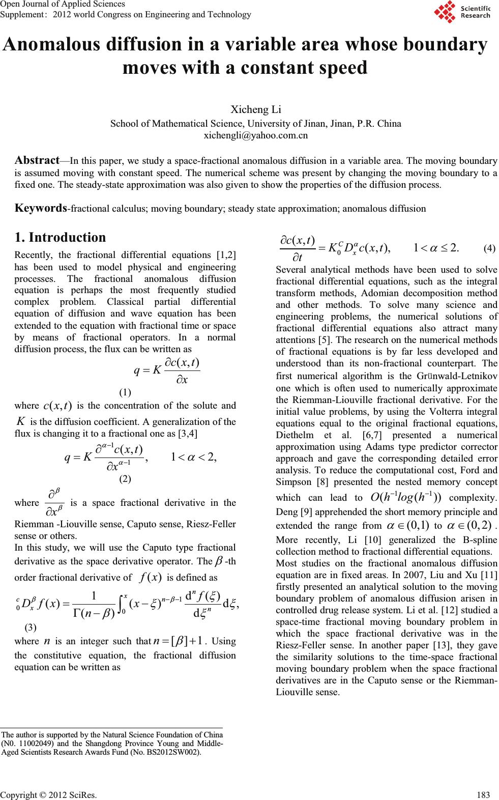Anomalous diffusion in a variable area whose boundary
moves with a constant speed
Xicheng Li
School of Mathematical Science, University of Jinan, Jinan, P.R. China
Abstract—In this paper, we study a space-fractional anomalous diffusion in a variable area. The moving boundary
is assumed moving with constant speed. The numerical scheme was present by changing the moving boundary to a
fixed one. The steady-state approximation was also given to show the properties of the diffusion process.
Keywords-fractional calculus; moving boundary; steady state approximation; anomalous diffusion
1. Introduction
Recently, the fractional differential equations [1,2]
has been used to model physical and engineering
processes. The fractional anomalous diffusion
equation is perhaps the most frequently studied
complex problem. Classical partial differential
equation of diffusion and wave equation has been
extended to the equation with fractional time or space
by means of fractional operators. In a normal
diffusion process, the flux can be written as
(,)cxt
qK x
w
w
(1)
where (,)cxt is the concentration of the solute and
K is the diffusion coefficient. A generalization of the
flux is changing it to a fractional one as [3,4]
1
1
(,)
,1 2,
cxt
qK x
D
DD


w

w
(2)
where
x
E
E
w
w
is a space fractional derivative in the
Riemman -Liouville sense, Caputo sense, Riesz-Feller
sense or others.
In this study, we will use the Caputo type fractional
derivative as the space derivative operator. The E -th
order fractional derivative of ()fx is defined as
1
00
1d()
()( )d,
() d
n
x
cn
xn
f
Dfxx
n
EE
[
[[
E[


* ³
(3)
where n is an integer such that []1n E  . Using
the constitutive equation, the fractional diffusion
equation can be written as
0
(,) (,), 12.
C
x
cxt KDcxt
t
DD
w d
w
(4)
Several analytical methods have been used to solve
fractional differential equations, such as the integral
transform methods, Adomian decomposition method
and other methods. To solve many science and
engineering problems, the numerical solutions of
fractional differential equations also attract many
attentions [5]. The research on the numerical methods
of fractional equations is by far less developed and
understood than its non-fractional counterpart. The
first numerical algorithm is the Grunwald-Letnikov
one which is often used to numerically approximate
the Riemman-Liouville fractional derivative. For the
initial value problems, by using the Volterra integral
equations equal to the original fractional equations,
Diethelm et al. [6,7] presented a numerical
approximation using Adams type predictor corrector
approach and gave the corresponding detailed error
analysis. To reduce the computational cost, Ford and
Simpson [8] presented the nested memory concept
which can lead to
11
(())Oh logh

complexity.
Deng [9] apprehended the short memory principle and
extended the range from (0,1) D  to (0,2) D  .
More recently, Li [10] generalized the B-spline
collection method to fractional differential equations.
Most studies on the fractional anomalous diffusion
equation are in fixed areas. In 2007, Liu and Xu [11]
firstly presented an analytical solution to the moving
boundary problem of anomalous diffusion arisen in
controlled drug release system. Li et al. [12] studied a
space-time fractional moving boundary problem in
which the space fractional derivative was in the
Riesz-Feller sense. In another paper [13], they gave
the similarity solutions to the time-space fractional
moving boundary problem when the space fractional
derivatives are in the Caputo sense or the Riemman-
Liouville sense.
The author is supported by the Natural Science Foundation of Chin
a
(N0. 11002049) and the Shangdong Province Young and Middle-
Aged Scientists Research Awards Fund (No. BS2012SW002).
Open Journal of Applied Sciences
Supplement：2012 world Congress on Engineering and Technology
Cop
y
ri
g
ht © 2012 SciRes.183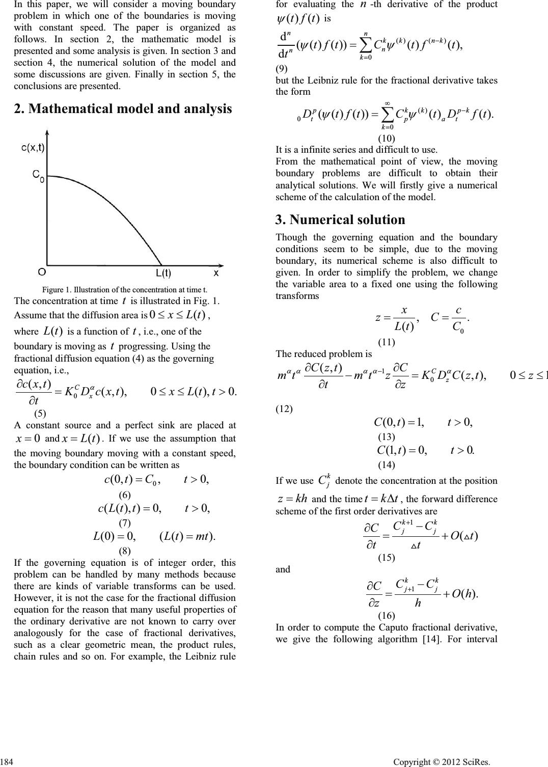

In this paper, we will consider a moving boundary
problem in which one of the boundaries is moving
with constant speed. The paper is organized as
follows. In section 2, the mathematic model is
presented and some analysis is given. In section 3 and
section 4, the numerical solution of the model and
some discussions are given. Finally in section 5, the
conclusions are presented.
2. Mathematical model and analysis
Figure 1. Illustration of the concentration at time t.
The concentration at time t is illustrated in Fig. 1.
Assume that the diffusion area is 0()xLtdd
,
where ()Lt is a function of t , i.e., one of the
boundary is moving as t
progressing. Using the
fractional diffusion equation (4) as the governing
equation, i.e.,
0
(,) (,),0( ),0.
C
x
cxt KDcxtxLt t
t
D
w dd!
w
(5)
A constant source and a perfect sink are placed at
0x
and
()xLt
. If we use the assumption that
the moving boundary moving with a constant speed,
the boundary condition can be written as
0
(0, ),0,ct Ct !
(6)
((),) 0,0,cLttt !
(7)
(0)0,(( )).LLtmt
(8)
If the governing equation is of integer order, this
problem can be handled by many methods because
there are kinds of variable transforms can be used.
However, it is not the case for the fractional diffusion
equation for the reason that many useful properties of
the ordinary derivative are not known to carry over
analogously for the case of fractional derivatives,
such as a clear geometric mean, the product rules,
chain rules and so on. For example, the Leibniz rule
for evaluating the n -th derivative of the product
() ()tft
\
is
()()
0
d( () ())()(),
d
nn
kk nk
n
n
k
tftCtf t
t
\\

¦
(9)
but the Leibniz rule for the fractional derivative takes
the form
()
0
0
( () ())()().
pkkpk
tpat
k
DtftC tDft \\
f
¦
(10)
It is a infinite series and difficult to use.
From the mathematical point of view, the moving
boundary problems are difficult to obtain their
analytical solutions. We will firstly give a numerical
scheme of the calculation of the model.
3. Numerical solution
Though the governing equation and the boundary
conditions seem to be simple, due to the moving
boundary, its numerical scheme is also difficult to
given. In order to simplify the problem, we change
the variable area to a fixed one using the following
transforms
0
,.
()
xc
zC
Lt C
(11)
The reduced problem is
1
0
(,)(,), 0
1
C
z
Czt C
mtmtzK DCztz
tz
DD DDD 
ww
 dd
ww
(12)
(0, )1,0,Ct t !
(13)
(1, )0,0.Ct t !
(14)
If we use
k
j
C denote the concentration at the position
zkh
and the time
tkt '
, the forward difference
scheme of the first order derivatives are
1
()
kk
jj
CC
COt
tt


w 
w+ +
(15)
and
1
().
kk
jj
CC
COh
zh


w 
w
(16)
In order to compute the Caputo fractional derivative,
we give the following algorithm [14]. For interval
184 Cop
y
ri
g
ht © 2012 SciRes.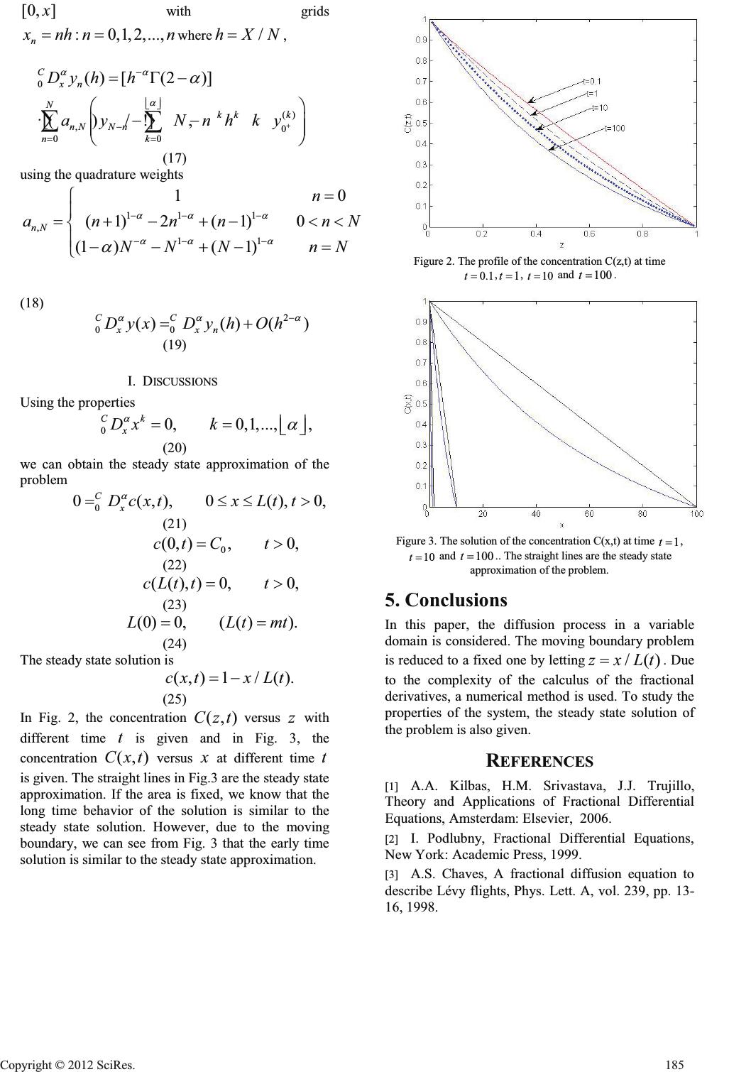

[0, ]x
with grids
: 0,1,2,...,
n
xnhn n where /hXN
,
0
()
,0
00
() [(2)]
·[()/ !],
C
xn
N
kk k
nNN n
nk
Dy hh
ay Nnhky
D
DD
D



¬¼
«»
*
§·

¨¸
¨¸
©¹
¦¦
(17)
using the quadrature weights
11 1
,
11
10
(1)2(1)0
(1 )(1)
nN
n
an nnnN
NN NnN
DD D
DD D
D
 
 

°

®
°
¯
(18)
2
00
()() ()
CC
xxn
DyxDy hOh
DD D 

(19)
I. DISCUSSIONS
Using the properties
0
0,0,1,..., ,
Ck
x
Dx k
D
D
«»
¬¼
(20)
we can obtain the steady state approximation of the
problem
0
0(,),0(),0,
C
x
DcxtxLt t
D
dd!
(21)
0
(0, ),0,ct Ct !
(22)
((),) 0,0,cLttt !
(23)
(0)0,(( )).LLtmt
(24)
The steady state solution is
(,)1/ ().cxtx Lt 
(25)
In Fig. 2, the concentration (,)Czt versus z with
different time t
is given and in Fig. 3, the
concentration (,)Cxt
versus
x
at different time
t
is given. The straight lines in Fig.3 are the steady state
approximation. If the area is fixed, we know that the
long time behavior of the solution is similar to the
steady state solution. However, due to the moving
boundary, we can see from Fig. 3 that the early time
solution is similar to the steady state approximation.
Figure 2. The profile of the concentration C(z,t) at time
0.1t
,
1t
,
10t
and
100t
.
Figure 3. The solution of the concentration C(x,t) at time
1t
,
10t
and
100t
.. The straight lines are the steady state
approximation of the problem.
5. Conclusions
In this paper, the diffusion process in a variable
domain is considered. The moving boundary problem
is reduced to a fixed one by letting /()zxLt . Due
to the complexity of the calculus of the fractional
derivatives, a numerical method is used. To study the
properties of the system, the steady state solution of
the problem is also given.
REFERENCES
[1] A.A. Kilbas, H.M. Srivastava, J.J. Trujillo,
Theory and Applications of Fractional Differential
Equations, Amsterdam: Elsevier, 2006.
[2] I. Podlubny, Fractional Differential Equations,
New York: Academic Press, 1999.
[3] A.S. Chaves, A fractional diffusion equation to
describe Lévy flights, Phys. Lett. A, vol. 239, pp. 13-
16, 1998.
Cop
y
ri
g
ht © 2012 SciRes.185

[4] P. Paradisi, R. Cesari, F. Mainardi, A. Maurizi
and F. Tampieri, A generalized Fick's law to describe
non-local transport effects, Physics and Chemistry of
the Earth, vol. 26, pp. 275-279, 2001.
[5] K. Dierhelm, N.J. Ford, A.D. Freed and Y.
Luchko, Algorithms for the fractional calculus: A
selection of numerical methods, Comput. Methods
Appl. Mech. Engrg, vol. 194, pp. 743-773, 2005.
[6] K. Diethelm, N.J. Ford, A.D. Freed, A predictor-
corrector approach for the numerical solution of
fractional differential equations, Nonlinear Dyn., vol.
29, pp. 3-22, 2002.
[7] K. Diethelm, N.J. Ford, A.D. Freed, Detailed
error analysis for a fractional Adams method. Numer.
Algorithms, vol. 36, pp. 31-52, 2004.
[8] N.J. Ford and A.C. Simpson, The numerical
solution of fractional differential equations: Speed
versus accuracy, Numerical Algorithms, vol. 26, pp.
333-346, 2001.
[9] W.H. Deng, Short memory principle and a
predictor-corrector approach for fractional differential
equations, J. Comput. Appl. Math. Vol. 206, pp. 174-
188, 2006.
[10] X.X. Li, Numerical solution of fractional
differential equations using cubic B-spline wavelet
collocation method, Commun Nonlinear Sci Numer
Simulat, vol. 17, pp. 3934–3946, 2012.
[11] J.Y. Liu and M.Y. Xu, Some exact solutions to
Stefan problems with fractional differential equations,
J. Math, Anal. Appl., vol. 351, pp. 536-542, 2009.
[12] X.C. Li, M.Y. Xu, S.W. Wang, Analytical
solutions to the moving boundary problems with
space-time-fractional derivatives in drug release
devices, Journal of Physics A: Mathematical and
Theoretical, vol. 40, pp. 12131-12141, 2007.
[13] X.C. Li, M.Y. Xu, S.W. Wang, Scale-invariant
solutions to partial differential equations of fractional
order with a moving boundary condition, Journal of
Physics A: Mathematical and Theoretical, vol. 41, pp.
155202, 2008.
[14] K. Diethelm, N.J. Ford, A.D. Freed and YU.
Luchko, Algorithms for the fractional calculus: A
selection of numerical methods, Comput. Methods
Appl. Mech. Engrg, vol. 194, pp. 743-773, 2005.
186 Cop
y
ri
g
ht © 2012 SciRes.