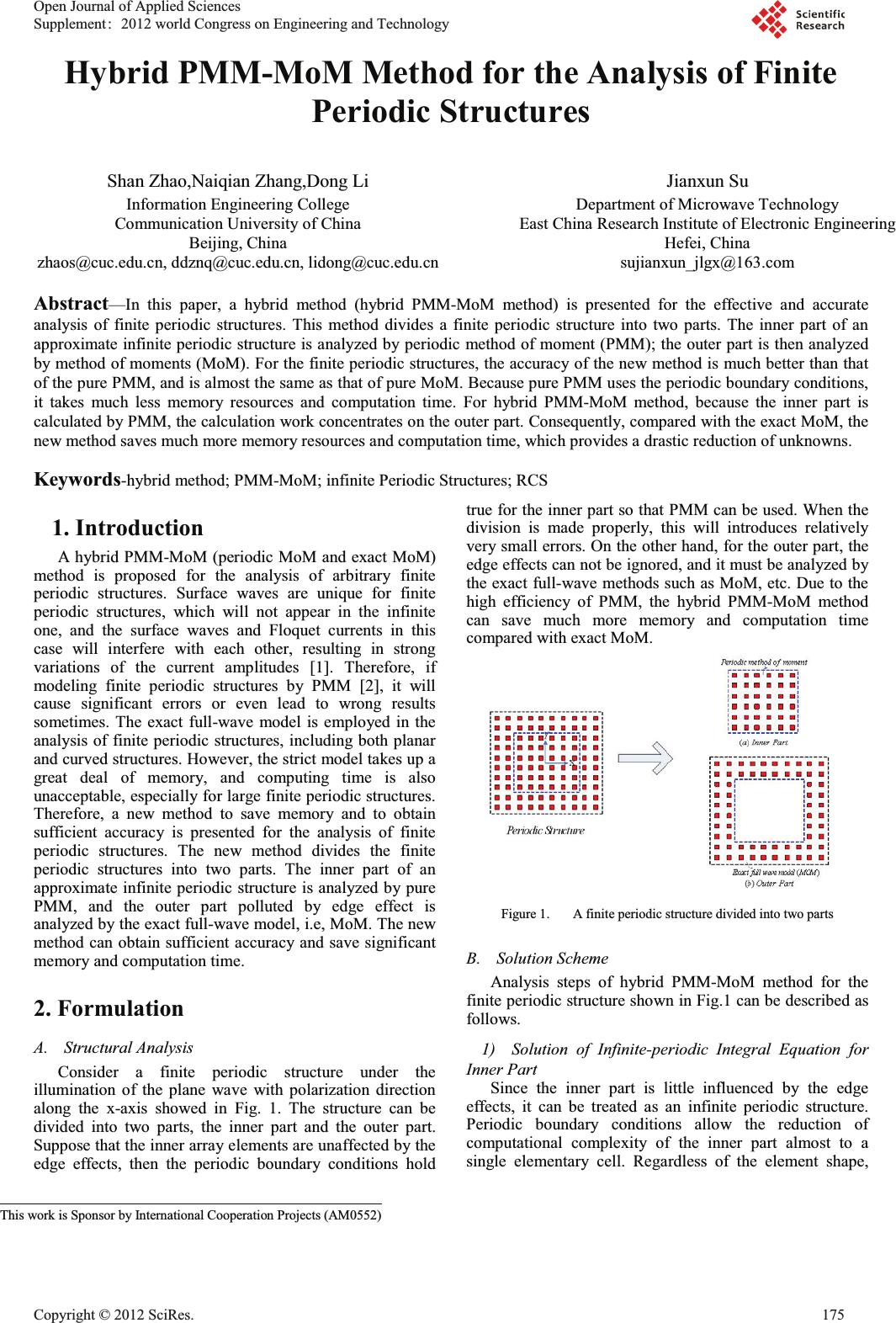Hybrid PMM-MoM Method for the Analysis of Finite
Periodic Structures
Shan Zhao,Naiqian Zhang,Dong Li
Information Engineering College
Communication University of China
Beijing, China
[e-mail], [e-mail], [e-mail]
Jianxun Su
Department of Microwave Technology
East China Research Institute of Electronic Engineering
Hefei, China
Abstract—In this paper, a hybrid method (hybrid PMM-MoM method) is presented for the effective and accurate
analysis of finite periodic structures. This method divides a finite periodic structure into two parts. The inner part of an
approximate infinite periodic structure is analyzed by periodic method of moment (PMM); the outer part is then analyzed
by method of moments (MoM). For the finite periodic structures, the accuracy of the new method is much better than that
of the pure PMM, and is almost the same as that of pure MoM. Because pure PMM uses the periodic boundary conditions,
it takes much less memory resources and computation time. For hybrid PMM-MoM method, because the inner part is
calculated by PMM, the calculation work concentrates on the outer part. Consequently, compared with the exact MoM, the
new method saves much more memory resources and computation time, which provides a drastic reduction of unknowns.
Keywords-hybrid method; PMM-MoM; infinite Periodic Structures; RCS
1. Introduction
A hybrid PMM-MoM (periodic MoM and exact MoM)
method is proposed for the analysis of arbitrary finite
periodic structures. Surface waves are unique for finite
periodic structures, which will not appear in the infinite
one, and the surface waves and Floquet currents in this
case will interfere with each other, resulting in strong
variations of the current amplitudes [1]. Therefore, if
modeling finite periodic structures by PMM [2], it will
cause significant errors or even lead to wrong results
sometimes. The exact full-wave model is employed in the
analysis of finite periodic structures, including both planar
and curved structures. However, the strict model takes up a
great deal of memory, and computing time is also
unacceptable, especially for large finite periodic structures.
Therefore, a new method to save memory and to obtain
sufficient accuracy is presented for the analysis of finite
periodic structures. The new method divides the finite
periodic structures into two parts. The inner part of an
approximate infinite periodic structure is analyzed by pure
PMM, and the outer part polluted by edge effect is
analyzed by the exact full-wave model, i.e, MoM. The new
method can obtain sufficient accuracy and save significant
memory and computation time.
2. Formulation
A.Structural Analysis
Consider a finite periodic structure under the
illumination of the plane wave with polarization direction
along the x-axis showed in Fig. 1. The structure can be
divided into two parts, the inner part and the outer part.
Suppose that the inner array elements are unaffected by the
edge effects, then the periodic boundary conditions hold
true for the inner part so that PMM can be used. When the
division is made properly, this will introduces relatively
very small errors. On the other hand, for the outer part, the
edge effects can not be ignored, and it must be analyzed by
the exact full-wave methods such as MoM, etc. Due to the
high efficiency of PMM, the hybrid PMM-MoM method
can save much more memory and computation time
compared with exact MoM.
Figure 1.A finite periodic structure divided into two parts
B.Solution Scheme
Analysis steps of hybrid PMM-MoM method for the
finite periodic structure shown in Fig.1 can be described as
follows.
1)Solution of Infinite-periodic Integral Equation for
Inner Part
Since the inner part is little influenced by the edge
effects, it can be treated as an infinite periodic structure.
Periodic boundary conditions allow the reduction of
computational complexity of the inner part almost to a
single elementary cell. Regardless of the element shape,
This work is Sponsor by International Cooperation Projects (AM0552)
Open Journal of Applied Sciences
Supplement：2012 world Congress on Engineering and Technology
Cop
y
ri
g
ht © 2012 SciRes.175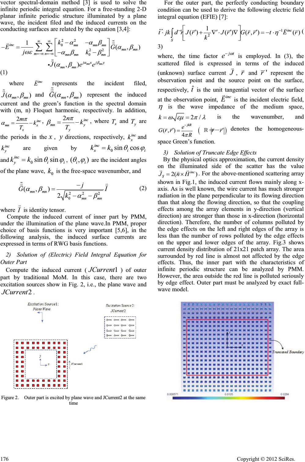

vector spectral-domain method [3] is used to solve the
infinite periodic integral equation. For a free-standing 2-D
planar infinite periodic structure illuminated by a plane
wave, the incident filed and the induced currents on the
conducting surfaces are related by the equation [3,4]:
22
0
22
0
1(,)
(,)
mn mn
inc mnmn mn
mn mn
mn mn mnmn
jxjy
mn mn
k
EG
jk
Jee
DE
DDE DE
ZH DE E
DE
ff
f f
ªº

 «»

¬¼
¦¦
K
K K
K

<
(1)
where
inc
E
K
represents the incident filed,
(,)
mn mn
J DE
K

and (,)
mn mn
G DE
K
K

represent the induced
current and the green’s function in the spectral domain
with (m, n) Floquet harmonic, respectively. In addition,
2
inc
mn x
x
mk
T
S
D 
,
2
inc
mn y
y
nk
T
S
E 
, where
x
T
and
y
T
are
the periods in the x , y directions, respectively, inc
x
kand
inc
y
k
are given by
0
sin cos
inc
xii
kk TM
and
0
sinsin
inc
yii
kk TM
,
(, )
ii
TM
are the incident angles
of the plane wave,
0
k is the free-space wavenumber, and
22 2
0
(,)
2
mn mn
mn mn
j
GI
k
DE DE


KK
KK

(2)
where
I
K
K
is identity tensor.
Compute the induced current of inner part by PMM,
under the illumination of the plane wave.In PMM, proper
choice of basis functions is very important [5,6], in the
following analysis, the induced surface currents are
expressed in terms of RWG basis functions.
2)Solution of (Electric) Field Integral Equation for
Outer Part
Compute the induced current ( 1JCurrent ) of outer
part by traditional MoM. In this case, there are two
excitation sources show in Fig. 2, i.e., the plane wave and
2JCurrent
.
Figure 2. Outer part is excited by plane wave and JCurrent2 at the same
time
For the outer part, the perfectly conducting boundary
condition can be used to derive the following electric field
integral equation (EFIE) [7]:
1
2
1
ˆˆ ()() (,)()
inc
S
tjkdrJrJrGrrtE r
k
K

ªº
cc ccc  
«»
¬¼
³
K
KKK KKK
(
3)
where, the time factor
jt
e
Z 
is employed. In (3), the
scattered filed is expressed in terms of the induced
(unknown) surface current J
K
, r
K
and 'r represent the
observation point and the source point on the surface,
respectively,
ˆ
t is the unit tangential vector of the surface
at the observation point, inc E
K is the incident electric field,
K
is the wave impedance of the medium space,
2/k ZHP SO
is the wavenumber, and

(, )4
jkR
e
Grrr r
R S

cc
KKKK
ǂˮ˙ˉ
denotes the homogeneous-
space Green’s function.
3)Solution of Truncate Edge Effects
By the physical optics approximation, the current density
on the illuminated side of the scatter has the value
2( )
inc
S
JnH u
KK
K
. For the above-mentioned scattering array
shown in Fig.1, the induced current flows mainly along x-
axis. As is well known, the wire current has much stronger
radiation in the plane perpendicular to its flowing direction
than that along the flowing direction, so that the coupling
effects among the array elements in y-direction (vertical
direction) are stronger than those in x-direction (horizontal
direction). Therefore, the number of columns polluted by
the edge effects on the left and right edges of the array is
less than the number of rows polluted by the edge effects
on the upper and lower edges of the array. Fig.3 shows
current density distribution of 21x21 patch array. The area
surrounded by red line is almost not affected by the edge
effects. Thus, the inner part with the characteristics of
infinite periodic structure can be analyzed by PMM.
However, the area outside the red line is polluted seriously
by edge effect. Outer part must be analyzed by exact full-
wave model.
176 Cop
y
ri
g
ht © 2012 SciRes.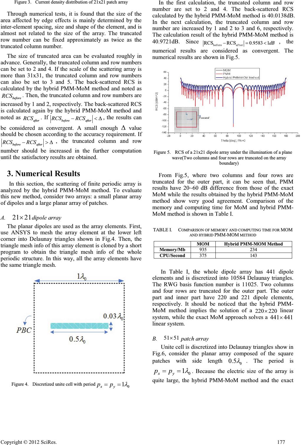

Figure 3.Current density distribution of 21x21 patch array
Through numerical tests, it is found that the size of the
area affected by edge effects is mainly determined by the
inter-element spacing, size and shape of the element, and is
almost not related to the size of the array. The truncated
row number can be fixed approximately as twice as the
truncated column number.
The size of truncated area can be evaluated roughly in
advance. Generally, the truncated column and row numbers
can be set to 2 and 4. If the scale of the scattering array is
more than 31x31, the truncated column and row numbers
can also be set to 3 and 5. The back-scattered RCS is
calculated by the hybrid PMM-MoM method and noted as
before
RCS
. Then, the truncated column and row numbers are
increased by 1 and 2, respectively. The back-scattered RCS
is calculated again by the hybrid PMM-MoM method and
noted as
after
RCS
. If
before after
RCS RCS'
, the results can
be considered as convergent. A small enough ' value
should be chosen according to the accuracy requirement. If
before after
RCS RCS!'
, the truncated column and row
number should be increased in the further computation
until the satisfactory results are obtained.
3. Numerical Results
In this section, the scattering of finite periodic array is
analyzed by the hybrid PMM-MoM method. To evaluate
this new method, consider two arrays: a small planar array
of dipoles and a large planar array of patches.
A. 21 21u dipole array
The planar dipoles are used as the array elements. First,
use ANSYS to mesh the array element at the lower left
corner into Delaunay triangles shown in Fig.4. Then, the
triangle mesh info of this array element is cloned by a short
program to obtain the triangle mesh info of the whole
periodic structure. In this way, all the array elements have
the same triangle mesh.
Figure 4.Discretized unite cell with period
0
1
xy
pp O
In the first calculation, the truncated column and row
number are set to 2 and 4. The back-scattered RCS
calculated by the hybrid PMM-MoM method is 40.0138dB.
In the next calculation, the truncated column and row
number are increased by 1 and 2 to 3 and 6, respectively.
The calculation result of the hybrid PMM-MoM method is
40.9721dB. Since
RCSRCS0.9583 1dB 
EHIRUH DIWHU
, the
numerical results are considered as convergent. The
numerical results are shown in Fig.5.
Figure 5.RCS of a 21x21 dipole array under the illumination of a plane
wave(Two columns and four rows are truncated on the array
boundary)
From Fig.5, where two columns and four rows are
truncated for the outer part, it can be seen that, PMM
results have 20~60 dB difference from those of the exact
MoM while the results obtained by the hybrid PMM-MoM
method show very good agreement. Comparison of the
memory and computing time for MoM and hybrid PMM-
MoM method is shown in Table ȱ.
TABLE I. COMPARISON OF MEMORY AND COMPUTING TIME FOR MOM
AND HYBRID PMM-MOM METHOD
MOMHybrid PMM-MOM Method
Memory/Mb 935 234
CPU/Second 375 143
In Table ȱ, the whole dipole array has 441 dipole
elements and is discretized into 10584 Delaunay triangles.
The RWG basis function number is 11025. Two columns
and four rows are truncated for the outer part. The outer
part and inner part have 220 and 221 dipole elements,
respectively. It should be noticed that the hybrid PMM-
MoM method implies the solution of a
220 220u
linear
system, while the exact MoM approach solves a 441 441u
linear system.
B.
51 51u
patch array
Unite cell is discretized into Delaunay triangles show in
Fig.6, consider the planar array composed of the square
patches with side length
0
0.5 O . The period is
0
1
xy
pp O
. Because the electric size of the array is
quite large, the hybrid PMM-MoM method and the exact
Cop
y
ri
g
ht © 2012 SciRes.177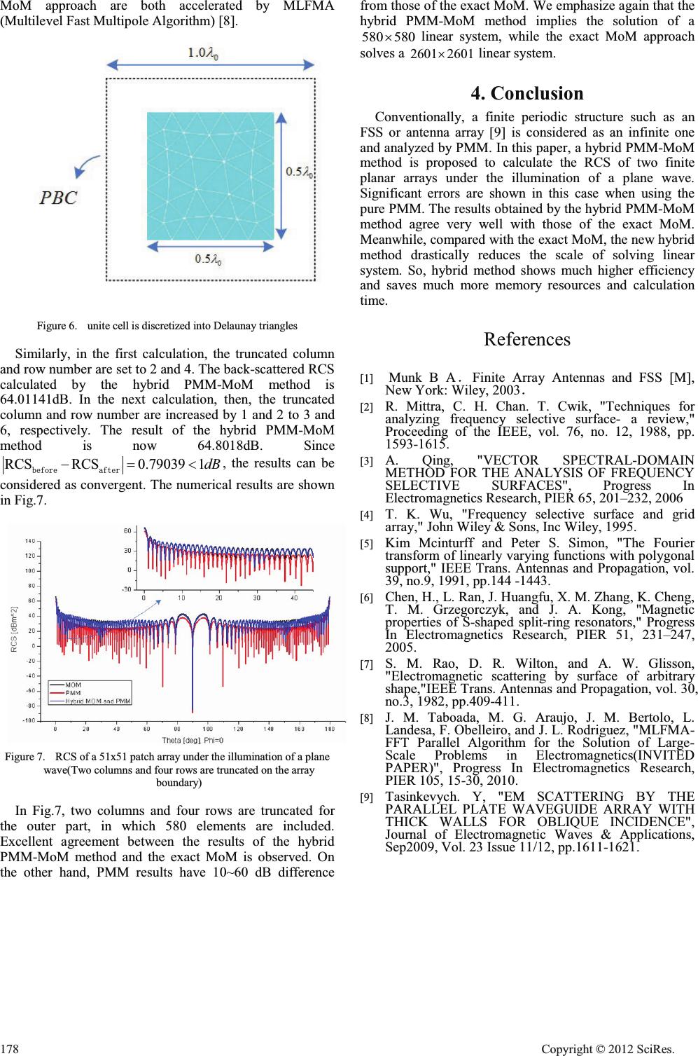

MoM approach are both accelerated by MLFMA
(Multilevel Fast Multipole Algorithm) [8].
Figure 6.unite cell is discretized into Delaunay triangles
Similarly, in the first calculation, the truncated column
and row number are set to 2 and 4. The back-scattered RCS
calculated by the hybrid PMM-MoM method is
64.01141dB. In the next calculation, then, the truncated
column and row number are increased by 1 and 2 to 3 and
6, respectively. The result of the hybrid PMM-MoM
method is now 64.8018dB. Since
RCSRCS0.790391dB 
EHIRUH DIWHU
, the results can be
considered as convergent. The numerical results are shown
in Fig.7.
Figure 7.RCS of a 51x51 patch array under the illumination of a plane
wave(Two columns and four rows are truncated on the array
boundary)
In Fig.7, two columns and four rows are truncated for
the outer part, in which 580 elements are included.
Excellent agreement between the results of the hybrid
PMM-MoM method and the exact MoM is observed. On
the other hand, PMM results have 10~60 dB difference
from those of the exact MoM. We emphasize again that the
hybrid PMM-MoM method implies the solution of a
580 580u
linear system, while the exact MoM approach
solves a 2601 2601u
linear system.
4. Conclusion
Conventionally, a finite periodic structure such as an
FSS or antenna array [9] is considered as an infinite one
and analyzed by PMM. In this paper, a hybrid PMM-MoM
method is proposed to calculate the RCS of two finite
planar arrays under the illumination of a plane wave.
Significant errors are shown in this case when using the
pure PMM. The results obtained by the hybrid PMM-MoM
method agree very well with those of the exact MoM.
Meanwhile, compared with the exact MoM, the new hybrid
method drastically reduces the scale of solving linear
system. So, hybrid method shows much higher efficiency
and saves much more memory resources and calculation
time.
References
[1] Munk B AˊFinite Array Antennas and FSS [M],
New York: Wiley, 2003ˊ
[2]R. Mittra, C. H. Chan. T. Cwik, "Techniques for
analyzing frequency selective surface- a review,"
Proceeding of the IEEE, vol. 76, no. 12, 1988, pp.
1593-1615.
[3]A. Qing, "VECTOR SPECTRAL-DOMAIN
METHOD FOR THE ANALYSIS OF FREQUENCY
SELECTIVE SURFACES", Progress In
Electromagnetics Research, PIER 65, 201–232, 2006
[4]T. K. Wu, "Frequency selective surface and grid
array," John Wiley & Sons, Inc Wiley, 1995.
[5]Kim Mcinturff and Peter S. Simon, "The Fourier
transform of linearly varying functions with polygonal
support," IEEE Trans. Antennas and Propagation, vol.
39, no.9, 1991, pp.144 -1443.
[6]Chen, H., L. Ran, J. Huangfu, X. M. Zhang, K. Cheng,
T. M. Grzegorczyk, and J. A. Kong, "Magnetic
properties of S-shaped split-ring resonators," Progress
In Electromagnetics Research, PIER 51, 231–247,
2005.
[7]S. M. Rao, D. R. Wilton, and A. W. Glisson,
"Electromagnetic scattering by surface of arbitrary
shape,"IEEE Trans. Antennas and Propagation, vol. 30,
no.3, 1982, pp.409-411.
[8]J. M. Taboada, M. G. Araujo, J. M. Bertolo, L.
Landesa, F. Obelleiro, and J. L. Rodriguez, "MLFMA-
FFT Parallel Algorithm for the Solution of Large-
Scale Problems in Electromagnetics(INVITED
PAPER)", Progress In Electromagnetics Research,
PIER 105, 15-30, 2010.
[9]Tasinkevych. Y, "EM SCATTERING BY THE
PARALLEL PLATE WAVEGUIDE ARRAY WITH
THICK WALLS FOR OBLIQUE INCIDENCE",
Journal of Electromagnetic Waves & Applications,
Sep2009, Vol. 23 Issue 11/12, pp.1611-1621.
178 Cop
y
ri
g
ht © 2012 SciRes.

Description of the derived categories of tubular algebras
in terms of dimension vectors
Hongbo Lv, Zhongmei Wang
School of Mathematical Science, University of Jinan, Jinan 250022, P.R.China
School of Control Science and Engineering, Shandong University, Jinan 250061, P.R.China
Abstract In this paper, we give a description of the derived category of a tubular algebra by calculating the dimension
vectors of the objects in it.
Keywords:derived categories; tubular algebra; dimension vectors
1.Introduction
Let
/
/
be a basic connected algebra over an algebraically
closed field k. We denote by mod/
/
the category of all
finitely generated right /
/
-modules and by ind /
/
a full
subcategory of mod /
/
containing exactly one
representative of each isomorphism class of
indecomposable /
/
-modules. For a /
/
-module M, we
denote the dimension vector by dim M. The bounded
derived category of mod
/
/
is denoted by Db(
/
/
). We
denote the Grothendieck group of /
/
by K0(/
/
), Auslander-
Reiten translation by W
W
, the Cartan matrix by
C
/
/
. Let

/
/
be the repetitive algebra of /
/
, mod

/
/
the stable module
category. When the global dimension of /
/
is finite,
C
/
/
is
invertible by [1], and Db( /
/
) is equivalent to mod

/
/
as
triangulated categories by [2].
By [1], a tubular extension A of a tame-concealed
algebra
of extension type T = (2, 2, 2, 2), (3, 3, 3), (4, 4, 2) or (6, 3,
2)
is called a tubular algebra. For example, the canonical
tubular algebras of T (2, 2, 2, 2) is determined by the
following quiver with relations.
By [1], global dimension of a tubular algebra A is 2, then
Db(A) is equivalent to mod
l
A
. And tubular algebras of the
same extension type are tilt-cotilt equivalent, see [3]. Then
we only consider the derived categories of canonical tubular
algebras, whose structures are given in [4].
 ()
b
r
rQ
DA T


where (1) for anyrෛ  Q, 7 r is the standard stable P1(k)-
tubular family of type T;
(2) for any r ෛQ, 7 r is separating
s
sr
T

 from u
ruT 
 .
Based on the results above, we give a description of the
derived category of a canonical tubular algebra by
calculating the dimension vectors of the objects in it.
2. Description of The Derived
Categories of Tubular Algebras In
Terms Of Dimension Vectors
In this section, let A be a canonical tubular algebra of
type T.
Definition 1.1. ([1]) Let n be the rank of Grothendieck
group K0(A),
A
C
the Cartan matrix of A. Then
(1) The Coxeter matrix A
) is defined by
T
AA
CC



(2) The quadratic form A F in
n
] is defined by
1
1
() ()
2
TT
AAA
CC FD DD


for any D in
n
] .
(3) Let 0,hh
fbe the positive generators of rad A
F . For an
A෥module M, define
0
(dim)
() (dim)
lM
index MlM
f

where
00
(dim )(dim ),
(dim )(dim ).
TT
A
TT
A
lMhC M
lMhC M


ff
In particular, for any
00
rad , ,
Arhrh
DFD
ff
 
where
0
0
,. Then, index().
r
rr r D
f
f
 ]
Open Journal of Applied Sciences
Supplement：2012 world Congress on Engineering and Technology
Cop
y
ri
g
ht © 2012 SciRes.179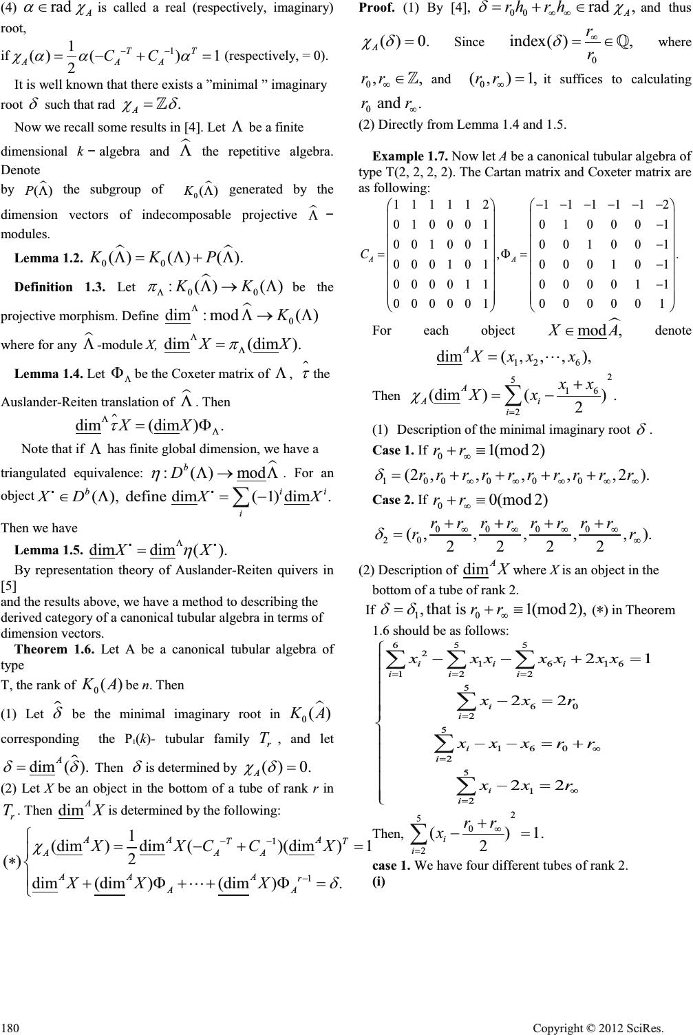

(4) rad
A
DF  is called a real (respectively, imaginary)
root,
if
1
1
()() 1
2
TT
AAA
CC FD DD


(respectively, = 0).
It is well known that there exists a ”minimal ” imaginary
root G such that rad .
A
FG ]
Now we recall some results in [4]. Let / be a finite
dimensional k෥algebra and
l
/
the repetitive algebra.
Denote
by
l
()P/
the subgroup of
l
0
()K/
generated by the
dimension vectors of indecomposable projective
l
/ ෥
modules.
Lemma 1.2.
ll
00
()() ().KKP/ //
Definition 1.3. Let
l
00
:() ()KK S
/
/o/ be the
projective morphism. Define
l
0
dim: mod()K
//o/
where for any
l
/ -module X, dim(dim ).XX S
/
/
Lemma 1.4. Let / )be the Coxeter matrix of
/
, W

the
Auslander-Reiten translation of
l
/ . Then
dim(dim ).XX
W
/
/
)

Note that if
/
has finite global dimension, we have a
triangulated equivalence:
l
:()mod
b
D
K
/o / . For an
object
(), define dim(1)dim.
bii
i
XDX X/ 
¦
<<
Then we have
Lemma 1.5. dimdim ().XX K
/
<<
By representation theory of Auslander-Reiten quivers in
[5]
and the results above, we have a method to describing the
derived category of a canonical tubular algebra in terms of
dimension vectors.
Theorem 1.6. Let A be a canonical tubular algebra of
type
T, the rank of 0()KA
be n. Then
(1) Let

G be the minimal imaginary root in
l
0()KA
corresponding the P1(k)- tubular family r T, and let

dim ().
A
GG Then G
is determined by ()0.
A
FG
(2) Let X be an object in the bottom of a tube of rank r in
r
T. Then
dimAX
is determined by the following:
1
1
1
(dim )dim ()(dim )1
2
()
dim(dim )(dim).
AA A
TT
AAA
AA A
r
AA
XXCCX
XX X
F
G


 
°
®
°))
¯"
Proof. (1) By [4], 00 rad ,
A
rhr h GF
ff
and thus
() 0.
A
FG Since
0
index( ),
r
r
G
f
_
where
0,,rr f] and 0
(,)1,rr
f
it suffices to calculating
0 and .rr f
(2) Directly from Lemma 1.4 and 1.5.
Example 1.7. Now let A be a canonical tubular algebra of
type T(2, 2, 2, 2). The Cartan matrix and Coxeter matrix are
as following:
111112 111112
0100010 10001
0010010 01001
,.
0001010 00101
000011 00001 1
000001 000001
AA
C

§·§·
¨¸¨¸

¨¸¨¸
¨¸¨¸

)
¨¸¨¸

¨¸¨¸
¨¸¨¸

¨¸¨¸
¨¸¨¸
©¹©¹
For each object
l
mod ,XA denote
12 6
dim( ,,,),
AXxx x "
Then
2
516
2
(dim)() .
2
A
Ai
i
xx
Xx F


¦
(1)Description of the minimal imaginary root G .
Case 1. If
01(mod 2)rr f
{
100000
(2,,,,,2).rr rr rr rr rr G
fffff

Case 2. If 00(mod 2)rr
f
{
0000
20
(,,,,,).
2222
rrrrrrrr
rr G
ffff
f

(2) Description of dimAX where X is an object in the
bottom of a tube of rank 2.
If 10
,that is 1(mod2),rr GG
f
{
(ѽ) in Theorem
1.6 should be as follows:
65 5
2
1616
12 2
5
60
2
5
160
2
5
1
2
21
22
22
iii
ii i
i
i
i
i
i
i
xxxxxxx
xx r
xxx rr
xxr
f
f

°
°
°
°
°
®
° 
°
°
°
°
¯
¦¦ ¦
¦
¦
¦
Then,
2
50
2
()1.
2
i
i
rr
xf


¦
case 1. We have four different tubes of rank 2.
(i)
180 Cop
y
ri
g
ht © 2012 SciRes.

00
0
00
11
dim(, , ,
22
11
,,)
22
Arr rr
Xr
rrrr r
ff
ff
f
 
 
00
0
00
11
dim(,,,
22
11
,,)
22
A
rr rr
Xr
rrrrr
W
ff
ff
f
 
 

(ii)
00
0
00
11
dim( ,,,
22
11
,,)
22
Arr rr
Xr
rrrr r
ff
ff
f
 
 
00
0
00
11
dim( ,,,
22
11
,,)
22
A
rr rr
Xr
rrrr r
W
ff
ff
f
 
 

(iii)
00
0
00
11
dim( ,,,
22
11
,,)
22
Arr rr
Xr
rrrr r
ff
ff
f
 
 
00
0
00
11
dim( ,,,
22
11
,,)
22
A
rr rr
Xr
rrrr r
W
ff
ff
f
 
 

(iv)
00
0
00
11
dim(1,,,
22
11
,,1)
22
A
rr rr
Xr
rrrr r
ff
ff
f
 

 
00
0
00
11
dim(1, , ,
22
11
,,1)
22
A
rr rr
Xr
rrrrr
W
ff
ff
f
 

 

If
2
, GG
(ѽ) in Theorem 1.6 should be as follows:
65 5
2
1616
12 2
5
60
2
50
16
2
5
1
2
21
2
2
2
iii
ii i
i
i
i
i
i
i
xxxxxxx
xxr
rr
xxx
xxr
f
f

°
°
°
°
°
®
°
°
°
°
°
¯
¦¦ ¦
¦
¦
¦
Then,
2
50
2
()1.
4
i
i
rr
xf


¦
case 2. When r0+r1 ิ2 (mod 4), we have four different
tubes of rank 2.
(i)
00 0
00
122
dim( ,,,
24 4
22 1
,,)
442
A
rrrrr
X
rr rr r
ff
ff f

 
00 0
00
122
dim( ,,,
24 4
22 1
,,)
442
Arrr rr
X
rr rr r
W
ff
ff f
 
 

(ii)
000
00
122
dim( ,,,
24 4
22 1
,,)
442
A
rrr rr
X
rr rr r
ff
ff f
 
 
00 0
00
122
dim( ,,,
24 4
22 1
,,)
442
A
rrr rr
X
rr rr r
W
ff
ff f
 
 

(iii)
000
00
122
dim(,,,
24 4
22 1
,,)
442
A
rrr rr
X
rr rr r
ff
ff f
 
 
000
00
122
dim(,,,
24 4
22
1
,,)
442
Arrr rr
X
rr rr r
W
ff
ff
f
 
 

(iv)
Cop
y
ri
g
ht © 2012 SciRes.181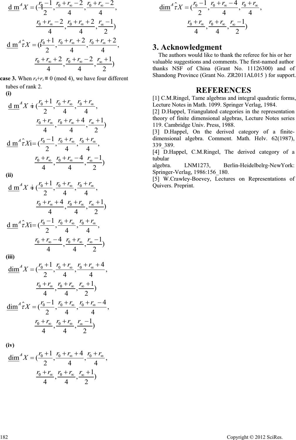

000
00
122
dim(,,,
24 4
22 1
,,)
442
A
rrr rr
X
rr rr r
ff
ff f
 
 
00 0
00
122
dim(,,,
24 4
22
1
,,)
442
A
rrr rr
X
rr rr r
W
ff
ff f
 
 

case 3. When r0+r1 ิ0 (mod 4), we have four different
tubes of rank 2.
(i)
00 0
00
1
dim(,,,
24 4
41
,,)
442
A
rrrrr
X
rrrr r
ff
ff f
 
 
00 0
00
1
dim(,,,
24 4
41
,,)
442
A
rrrrr
X
rrrr r
W
ff
ff f




(ii)
00 0
00
1
dim(,,,
24 4
41
,,)
442
Arrrrr
X
rr rr
r
ff
ff f
 
 
00 0
00
1
dim(,,,
24 4
41
,,)
442
A
rrrrr
X
rr rr
r
W
ff
ff f

 

(iii)
00 0
00
14
dim( ,,,
24 4
1
,,)
442
A
rrrrr
X
rrrr
r
ff
ff f
 

00 0
00
14
dim( ,,,
244
1
,,)
442
A
rrrrr
X
rrrr
r
W
ff
ff f
 


(iv)
00 0
00
14
dim( ,,,
24 4
1
,,)
442
A
rrr rr
X
rrrr r
ff
ff
f
 

000
00
14
dim( ,,,
24 4
1
,,)
442
A
rrr rr
X
rrrr r
W
ff
ff f
 


3. Acknowledgment
The authors would like to thank the referee for his or her
valuable suggestions and comments. The first-named author
thanks NSF of China (Grant No. 11126300) and of
Shandong Province (Grant No. ZR2011AL015 ) for support.
REFERENCES
[1] C.M.Ringel, Tame algebras and integral quadratic forms,
Lecture Notes in Math. 1099. Springer Verlag, 1984.
[2] D.Happel, Triangulated categories in the representation
theory of finite dimensional algebras, Lecture Notes series
119. Cambridge Univ. Press, 1988.
[3] D.Happel, On the derived category of a finite-
dimensional algebra. Comment. Math. Helv. 62(1987),
339_389.
[4] D.Happel, C.M.Ringel, The derived category of a
tubular
algebra. LNM1273, Berlin-Heidelbelrg-NewYork:
Springer-Verlag, 1986:156_180.
[5] W.Crawley-Boevey, Lectures on Representations of
Quivers. Preprint.
182 Cop
y
ri
g
ht © 2012 SciRes.