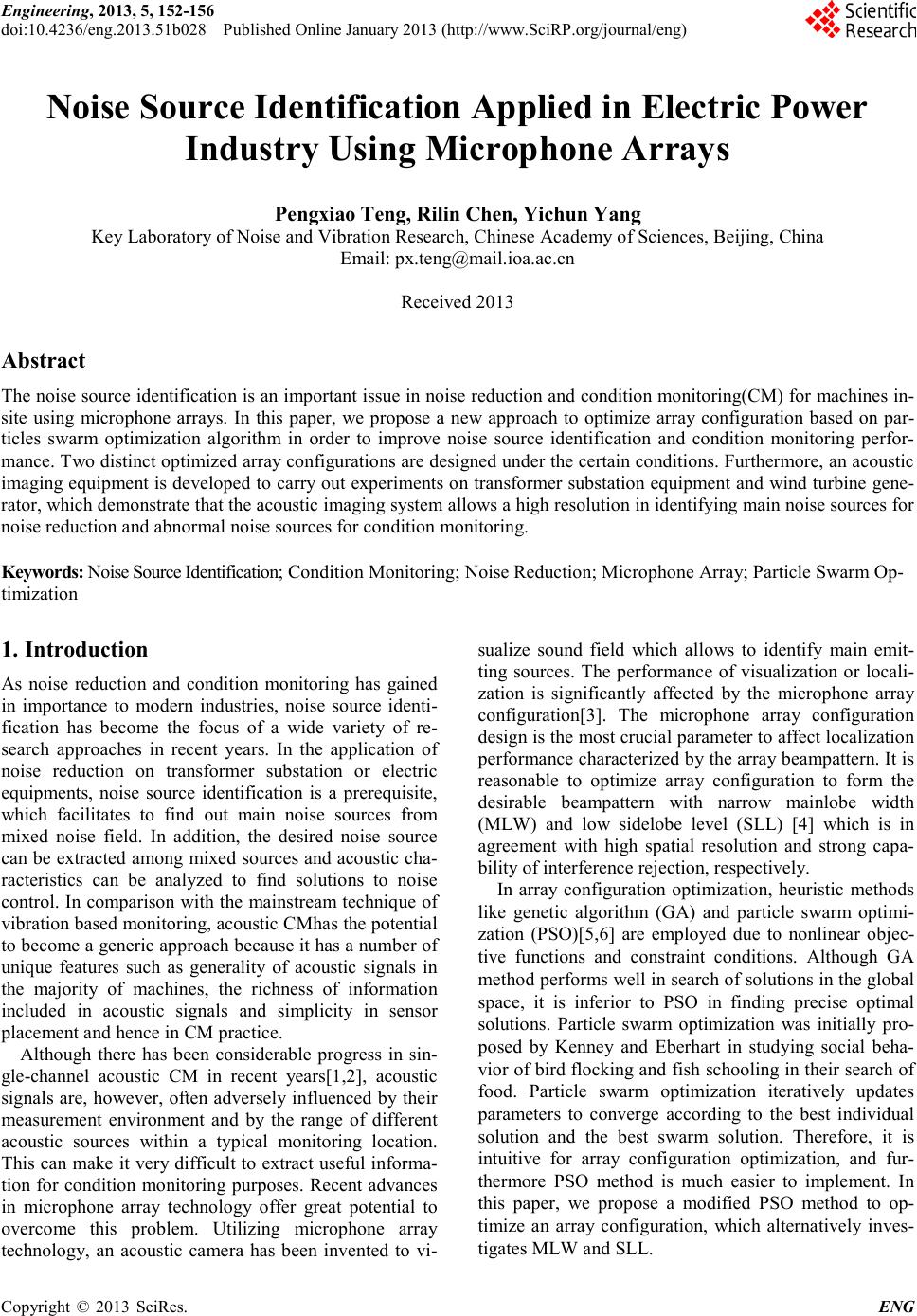Engineering, 2013, 5, 152-156
doi:10.4236/eng.2013.51b028 Published Online January 2013 (http://www.SciRP.org/journal/eng)
Noise Source Identification Applied in Electric Power
Industry Using Microphone Arrays
Pengxiao Teng, Rilin Chen, Yichun Yang
Key Laboratory of Noise and Vibration Research, Chinese Acad emy of Scie nces, Beijing, China
Received 2013
Abstract
The noise source identification is an i mportant issue in noise reductio n and co ndition monitoring(CM) for machines in-
site using microphone arrays. In this paper, we propose a new approach to optimize array configuration based on par-
ticles swarm optimization algor ith m in order to improve noise source identification and condition monitoring perfor-
mance. T wo distinct opti mized array configuratio ns are designed under the certain conditions. Furthermore, an aco ustic
imagi ng equi pment is d eveloped to carry out experiments on transformer subs tation equipment and wind turbine gene-
rator, which d e monstrate t hat the ac ous tic i ma gi ng s yst e m a llo ws a high resolutio n in id ent ifyi ng main no ise sour ces fo r
noise reduction and abnormal noise sources for condition mo nitorin g.
Keywords: Noise Source Identification; Condition Monitoring; Noise Reduction; Microphone Arra y; Particle Swarm Op-
timization
1. Introduction
As noise reduction and condition monitoring has gained
in importance to modern industries, noise source identi-
fication has become the focus of a wide variety of re-
search approaches in recent years. In the application of
noise reduction on transformer substation or electric
equipments, noise source identification is a prerequisite,
which facilitates to find out main noise sources from
mixed noise field. In addition, the desired noise source
can be extracted among mixed sources and acoustic cha-
racteristics can be analyzed to find solutions to noise
control. In compar ison with the mainstr eam tec hnique o f
vibration based monitoring, acoustic CMhas the po tentia l
to become a generic approach because it has a number of
unique features such as generality of acoustic signals in
the majority of machines, the richness of information
included in acoustic signals and simplicity in sensor
placement and hence in CM practice.
Although there has been considerable progress in sin-
gle-channel acoustic CM in recent years[1,2], acoustic
signals are, however, often adversely influenced by their
measurement environment and by the range of different
acoustic sources within a typical monitoring location.
This can make it very difficult to extra ct useful informa-
tion for condition monitoring purposes. Recent advances
in microphone array technology offer great potential to
overcome this problem. Utilizing microphone array
technology, an acoustic camera has been invented to vi-
sualize sound field which allows to identify main emit-
ting sources. The performance of visualization or locali-
zation is significantly affected by the microphone array
configuration[3]. The microphone array configuration
design is the most crucial p arameter to affect localiza tion
performance characterized b y the array beampattern. It is
reasonable to optimize array configuration to form the
desirable beampattern with narrow mainlobe width
(MLW) and low sidelobe level (SLL) [4] which is in
agreement with high spatial resolution and strong capa-
bility of interference rejection, respectively.
In array configuration optimization, heuristic methods
like genetic algorithm (GA) and particle swarm optimi-
zation (PSO)[5,6] are employed due to nonlinear objec-
tive functions and constraint conditions. Although GA
method pe rfor ms well i n sea rch o f solut io ns in the glob al
space, it is inferior to PSO in finding precise optimal
solutions. Particle swarm optimization was initially pro-
posed by Kenney and Eberhart in studying social beha-
vior o f bird flo cking a nd fish school ing in t heir sea rch of
food. Particle swarm optimization iteratively updates
parameters to converge according to the best individual
solution and the best swarm solution. Therefore, it is
intuitive for array configuration optimization, and fur-
thermore PSO method is much easier to implement. In
this paper, we propose a modified PSO method to op-
timize an array configuration, which alternatively inves-
tigates MLW and SLL.

P. X. TENG ET AL.
153
This paper is organize as follows. In Sect.2, we give
the array configuration model. A modified PSO method
is proposed to optimize two distinct array configuration
in Sect.3. We develop an acoustic imaging system and
carry out experiments in Sect.4 and the conclusion are
drawn in Sect. 5.
2. Array Model
As is known that the noise so urce identification is hig hly
related to the array beampattern, the beampattern formu-
la is given for the designed array, and then an modified
PSO method is proposed to optimize array configuration
both according to MLW and SLL in thi s s ectio n.
2.1. Planar Array Model
Figure 1 . Planar array model
Spiral arrays are widely used due to the merit of low
sidelobe. We optimize an array configuration based on
spiral structure. Assume that a source signal propagates
from the direction
(,) θϕ
and the coordinate of micro-
phone
m
p
is
[ cos,sin]
mmm m
rr φφ
. The time delay of
m
th micr ophone is represented as:
( )()
cossin cossinsin sin
m
mm
r
m
c
τφθϕ φθϕ
= +
(1)
Usin g Eqatio n (1) , one may obtain the beampattern as:
( )
1
cossin cos
,exp sinsin sin
Mm
m
m
mm
r
B wj
c
φ θϕ
ω
θϕ φ θϕ
=
=+
 
 
 
∑
(2)
2.2. 3D Array Model
Considering practical applications in imaging large
machine acou stically in a reve rb era nt ind ustrial pla nt, we
design a 3D microphone array with 8 arms at which 8
microphones are installed. An eight-arm 3D microphone
array is illustrated in Figure 2. The angle between the lth
arm and z axis is denoted as
( )
,1, 2,,
l
lL ϑ =
and the
angle between the projection of the lth arm on the xoy
plane and x axis is
( )
,1, 2,,
l
lL
φ =. The time delay of
l
m
th microphone at lth arm is represented by Eqation
(3), where
( )
,1, 2,,;1, 2,,
l
lm
ll
rl LmM= =

is de-
fined as the distance from the ml th microphone to the
coordinate origin. Ml is the number of microphone at lth
arm and
c
is sound velocity. Using Eqa tio n (3) , one
may obtain the beampattern by Euq ation (4), where
ω
is the signal frequency and
l
lm
w
is the weight. Without
loss of ge nerality, all weights are set to one.
The MLW is defined as Θ which is the angular inter-
val of the first pair nulls of
( )
|,
|B θϕ
for a given
ϕ
and the sid elob e level is represented as:
( )
( )
10
max
SSL
,
20log ,
B
B
θϕ
θϕ
∉Θ
=
(5)
where ∉Θ means sidelobe which is the angular interval
outside the mainlobe. Based on the narrow MLW and
low SLL criterion, an array configuration can be opti-
mized by
( )
( )
1 minmax
0 max0
1
0
min {MLW,max{SLL}}
.. ,
1
1,1, 0.
ll
ll
l lM
lml l
l
ll
m
st rrrr
r rrrMmr
l LmMr
+
= =
+≤≤−−−
≤≤≤≤>
，
，
(6)
where
1 min
l
l
rr=
and
max
l
lM
rr=
, with [
min
r
,max
r
]
being the distance interva l within which microp hones are
deployed. We also constrain the distance between two
adjacent microphones is larger than
0
r
. I n this p a p er, we
employ PSO method to implement the optimization.
( )()
,sincossin cossinsinsin sincoscos
l
lm
llllll
r
lm
c
τϑφθϕ ϑφθϕϑθ
= ++
(3)
( )()
11
,expsincossin cossinsinsin sincoscos
l
l
l
l
Llm
lm lllll
l
M
m
r
B wj
c
ω
θϕϑφθϕ ϑφθϕϑθ
= =
= ++



∑∑
(4)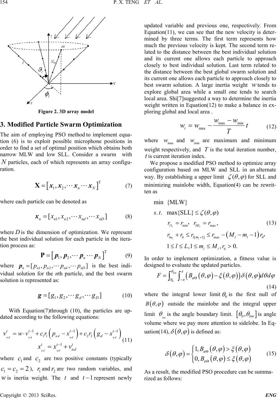

P. X. TENG ET AL.
154
Figure 2. 3D array model
3. Modified Particle Swarm Optimization
The aim of employing PSO method to implement equa-
tion (6) is to exploit possible microphone positions in
order to find a set of optimal position which obtains both
narrow MLW and low SLL. Consider a swarm with
N
particles, each of which represents an array configu-
ration.
[ ]
T
12
,, nN =Xxxx x
(7)
where each particle can be denoted as
12
[, ,,]
nn nndnD
xx x x=x (8)
where
D
is the dimension of optimization. We represent
the best individual solut ion for each particle in the itera-
tion process as:
[ ]
T
12
,, nN =Pppp p
(9)
where
12
[, ,,]
nn nndnD
pp p p=p
is the best indi-
vidual solution for the nth particle, and the best swarm
solution is represented as:
12
[, ,,]
dD
gg gg=g
(10)
With Equation(7)through (10), the particles are up-
dated ac c ording to the following equations:
() ()
112 2
11 1
1
nd ndndnd
ndnd
nd
tt tt
d
ttt
nd
w vcrpxcrgxv
xxv
−− −
−
=⋅+− +−
= +
(11)
where
1
c
and 2 c are two positive constants (typically
12
2 cc= =
),
1
r
and
2
r
are two random variables, and
w
is inertia weight. The
t
and
1t−
represent newly
updated variable and previous one, respectively. From
Equation(11), we can see that the new velocity is deter-
mined by three terms. The first term represents how
much the previous velocity is kept. The second term re-
lated to the distance between the best indi vidual so lutio n
and its current one allows each particle to approach
closely to best individual solution. Last term related to
the distance between the best global swarm solution and
its current one allows each particle to approach closely to
best swarm solution. A large inertia weight
w
tends to
explore global area while a small one tends to search
local area. Shi[7]suggested a way to d etermine the inertia
weight written in Equation(12) to make a balance in ex-
ploring global and local area .
max min
maxt
ww
ww t
T
−
= −
(12)
where
max
w
and min ware maximum and minimum
weight respectively, and
T
is the total iteration number,
t
is current iterat ion inde x.
We p rop ose a modified PSO method to optimize array
configuration based on MLW and SLL in an alternate
way. B y establishin g a uppe r limit
(,) ζθϕ
for SLL and
minimizing mainlobe width, Equation(4) can be rewrit-
ten as
( )
( )
1 minmax
0 max0 1
0
min {MLW}
. .max{SLL}(,)
,
1
1,1, 0.
ll
ll
l lM
lml l l
ll
m
st
rrr r
r rrrMmr
l LmMr
ζθϕ
+
≤
= =
+≤≤−−−
≤≤≤≤>
，
，
(13)
In order to implement optimization, a fitness value is
designed to evaluate the updated particles.
( )( ) ( ) ( )
0
, ,,
lim
F Bdd
θπ
θπ
θϕξθϕδ θϕθϕ
∉Θ
−
= −
∫∫
(14)
where the integral lower limit
0
θ
is the first null of
( )
,B θϕ
outside the mainlobe and the integral upper
limit
lim
θ
is the angle boundary limit.
[ ]
0,lim
θθ is angle
volume where we pay more attention to sidelobe. In Eq-
uation(14),
( )
, δ θϕ
is defined as:
( )( )( )
( )()
1, ,,
,0, ,,
B
B
θϕ ξθϕ
δ θϕθϕ ξθϕ
∉Θ
∉Θ
> 

=≤


(15)
As a result, the modified PSO procedure can be summa-
rized as follows: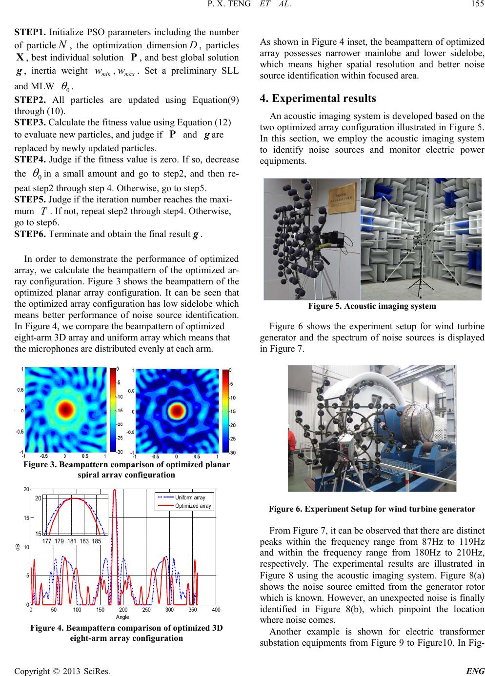

P. X. TENG ET AL.
155
STEP1. Initialize PSO parameters including the number
of particle
N
, the optimization dimension
D
, particles
X
, best individual sol utio n
P
, and best global solution
g
, inertia weight
min
w
,
max
w
. Set a preliminary SLL
and MLW 0
θ
.
STEP2. All particles are updated using Equation(9)
through (10).
STEP3. Calculate the fitness value using Equation (12)
to evaluate new particles, and j udge if
P
and
g
are
replaced by newly updated particles.
STEP4. Judge if the fitness value is zero. If so, decrease
the
0
θ
in a small amount and go to step2, and then re-
peat step2 through step 4. Otherwise, go to step5.
STEP5. Judge if the iteration number reaches the maxi-
mum
T
. If not, repeat step2 through step4. Otherwise,
go to step6.
STEP6. T erminate and obtain the final result
g
.
In order to demonstrate the performance of optimized
array, we calculate the beampattern of the optimized ar-
ray configuration. Figure 3 shows the beampattern of the
optimized planar array configuration. It can be seen that
the optimized array configuratio n has low sidelobe which
means better performance of noise source identification.
In Figure 4, we compare the beampattern of optimized
eight-ar m 3D array and uniform arra y which means that
the microphon es are dist ributed even ly at each arm.
Figure 3. Beampatt ern co mparison o f optimized planar
spir al array configuration
Figure 3. Beampat ter n o f opti m ized planar s pir al
array configuration
Figure 4. Beampat ter n comparison of optimized 3D
eig ht-arm array configuration
As shown in Figur e 4 inset, the beampattern of optimized
array possesses narrower mainlobe and lower sidelobe,
which means higher spatial resolution and better noise
source identification within focused area.
4. Experimental results
An acoustic imaging system is developed based on the
two optimized array configuration illustrated in Figure 5.
In this section, we employ the acoustic imaging system
to identify noise sources and monitor electric power
equipments.
Figure 5. Acoustic imaging system
Figure 6 shows the experiment setup for wind turbine
generator and the spectrum of noise sources is displayed
in Figure 7.
Figure 6. Experiment Setup for wi nd turbine generator
From Figure 7, it can be observed that there are distinct
peaks within the frequency range fro m 87Hz to 119Hz
and within the frequency range from 180Hz to 210Hz,
respectively. The experimental results are illustrated in
Figure 8 using the acoustic imaging system. Figure 8(a)
shows the noise source emitted from the generator rotor
which is kno wn. Ho wever , an unexpected noise is finally
identified in Figure 8(b), which pinpoint the location
where noise comes.
Another example is shown for electric transformer
substation equipments from Figure 9 to Figure10. In Fig-
050100 150 200 250 300 350 400
0
5
10
15
20
A ngle
dB
Uniform array
Opt i m i zed array
177 179181 183 185
15
20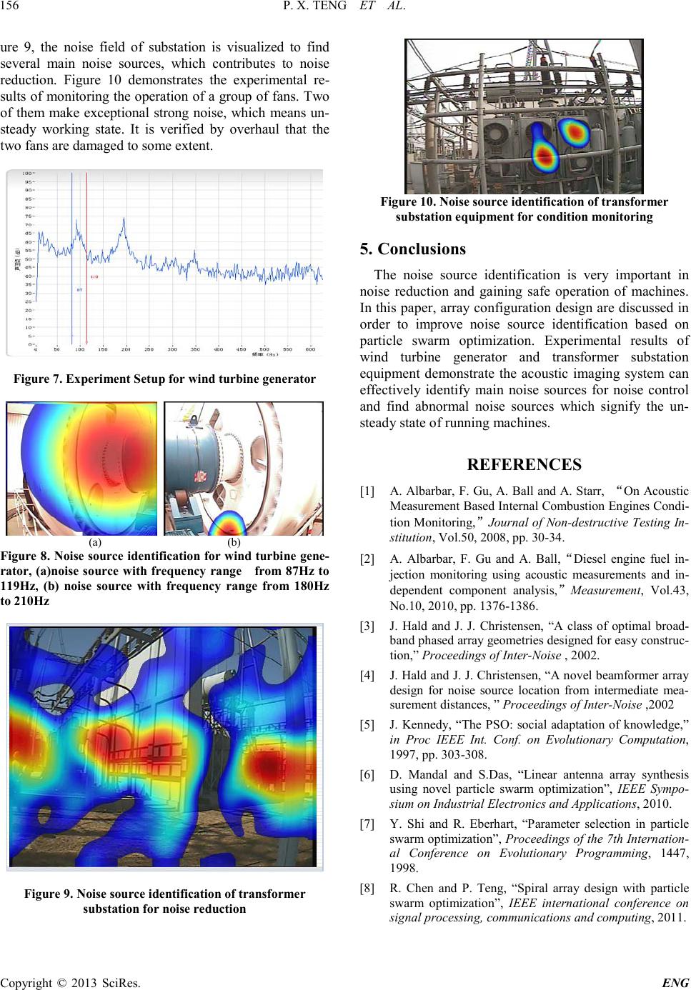

P. X. TENG ET AL.
156
ure 9, the noise field of substation is visualized to find
several main noise sources, which contributes to noise
reduction. Figure 10 demonstrates the experimental re-
sults of monitoring the operation of a group of fans. Two
of them make exceptional strong noise, which means un-
steady working state. It is verified by overhaul that the
two fans ar e d amaged to some extent.
Figure 7. Expe ri ment Setup for wi nd turbine generator
(a) (b)
Figure 8. Noise sourc e ident ificat ion for w ind turbi ne gene-
rator, (a)noise source with frequency range from 87Hz to
119Hz, (b) noise source with frequency range from 180Hz
to 210Hz
Figure 9. Noise source identifi cat ion of transformer
substation for noise reduction
Figure 10. Noise source identif icat ion of transformer
substation equi pme nt for co ndition monitoring
5. Conclusions
The noise source identification is very important in
noise reduction and gaining safe operation of machines.
In this paper, array configuration design are discussed in
order to improve noise source identification based on
particle swarm optimization. Experimental results of
wind turbine generator and transformer substation
equipment demonstrate the acoustic imaging system can
effectively identify main noise sources for noise control
and find abnormal noise sources which signify the un-
steady state of running machines.
REFERENCES
[1] A. Alb arbar, F. Gu, A. Ball and A. Starr, “On Acoustic
Measurement Based Internal Combustion Engines Condi-
tion Monitoring,”Journal o f Non-d estructive Testing In-
stitution, Vol.50, 2008, pp. 30-34.
[2] A. Albarbar, F. Gu and A. Ball,“Diesel engine fuel in-
jection monitoring using acoustic measurements and in-
dependent component analysis,”Measurement, Vol . 43,
No.10, 20 10, pp. 1376-1386.
[3] J. Hald and J. J. Christensen, “A class of optimal broad-
band phased array geometr ies d es igned for eas y co ns tru c-
tion,” Proceedings of Inter-Noise , 2002.
[4] J. Hald and J. J . Christen sen, “A novel b eamformer arra y
design for noise source location from intermediate mea-
surement distan ces , ” Proceedings of Inter-Noise ,2002
[5] J. Kennedy, “The PSO: social adaptation of knowledge,”
in Proc IEEE Int. Conf. on Evolutionary Computation,
1997, pp . 303-308.
[6] D. Mandal and S.Das, “Linear antenna array synthesis
using novel particle swarm optimization”, IEEE Sympo-
sium on Industrial Electronics and Applications, 2010.
[7] Y. Shi and R. Eberhart, “Parameter selection in particle
swarm optimization”, Proceedings of the 7th Internation-
al Conference on Evolutionary Programming, 1447,
1998.
[8] R. Chen and P. Teng, “Spiral array design with particle
swarm optimization”, IEEE international conference on
signal processing, communications and computing, 2011.