Paper Menu >>
Journal Menu >>
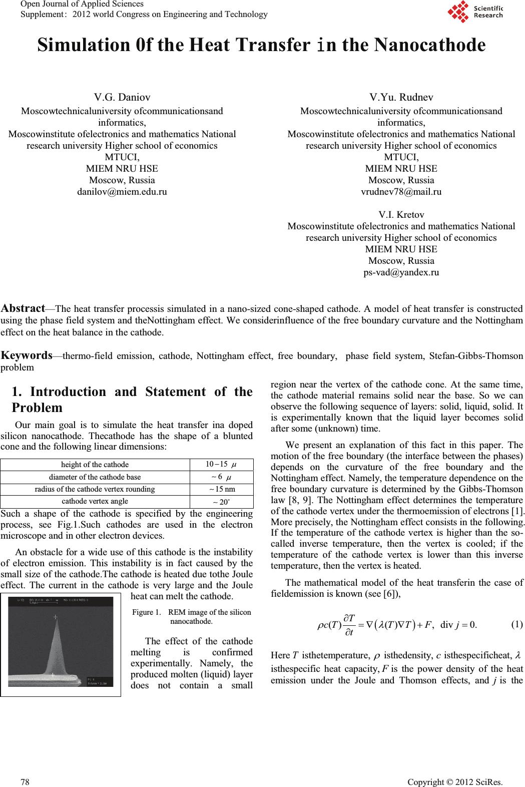 Simulation 0fthe Heat Transfer L n the Nanocathode V.G. Daniov Moscowtechnicaluniversity ofcommunicationsand informatics, Moscowinstitute ofelectronics and mathematics National research university Higher school of economics MTUCI, MIEM NRU HSE Moscow, Russia danilov@miem.edu.ru V.Yu. Rudnev Moscowtechnicaluniversity ofcommunicationsand informatics, Moscowinstitute ofelectronics and mathematics National research university Higher school of economics MTUCI, MIEM NRU HSE Moscow, Russia vrudnev78@mail.ru V.I. Kretov Moscowinstitute ofelectronics and mathematics National research university Higher school of economics MIEM NRU HSE Moscow, Russia ps-vad@yandex.ru Abstract—The heat transfer processis simulated in a nano-sized cone-shaped cathode. A model of heat transfer is constructed using the phase field system and theNottingham effect. We considerinfluence of the free boundary curvatureand the Nottingham effect on the heat balance in the cathode. Keywords—thermo-field emission, cathode, Nottingham effect, free boundary, phase field system, Stefan-Gibbs-Thomson problem 1. Introduction and Statement of the Problem Our main goal is to simulate the heat transfer ina doped silicon nanocathode. Thecathode has the shape of a blunted cone and the following linear dimensions: height of the cathode 10 15 P diameter of the cathode base 6 P radius of thecathode vertex rounding 15 nm cathode vertex angle 20 D Such a shape of the cathode is specified by the engineering process, see Fig.1.Such cathodes are used in the electron microscope and in other electron devices. An obstacle for a wide use of this cathode is the instability of electron emission. This instability is in fact caused by the small size of the cathode.The cathode is heated due tothe Joule effect. The current in the cathode is very large and the Joule heat can melt the cathode. Figure 1. REM image of the silicon nanocathode. The effect of the cathode melting is confirmed experimentally. Namely, the produced molten(liquid) layer does not contain a small region near the vertex of the cathode cone. At the same time, the cathode material remains solid near the base. So we can observe the following sequence oflayers: solid, liquid, solid. It is experimentally known that the liquid layer becomes solid after some (unknown) time. We present anexplanation of this fact in thispaper. The motion of the free boundary (the interface between the phases) depends on the curvature of the free boundary and the Nottingham effect. Namely, the temperature dependence on the free boundary curvature is determined by the Gibbs-Thomson law [8, 9]. The Nottingham effect determines the temperature of the cathode vertex under the thermoemission of electrons [1]. More precisely, the Nottingham effect consists in the following. If the temperature of the cathode vertex is higher than the so- called inverse temperature, then the vertex is cooled;if the temperature of the cathode vertex is lower than this inverse temperature, then the vertex is heated. The mathematical model of the heat transferin the case of fieldemission is known (see [6]), ()() , T cTT TF t UO w w div 0.j Here T isthetemperature, U isthedensity, c isthespecificheat, O isthespecific heat capacity,Fis the power density of the heat emission under the Joule and Thomson effects, and j is the Open Journal of Applied Sciences Supplement:2012 world Congress on Engineering and Technology 78 Cop y ri g ht © 2012 SciRes. 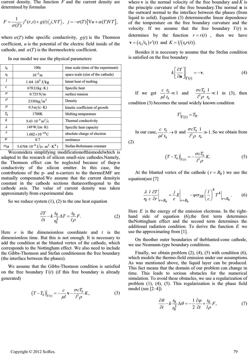 current density. The function Fand the current density are determined by formulas 2 1(,)() ,, () FjrtgtjT T V >@ ()() ,jTuTT VD where ()T V isthe specific conductivity, ()gt is the Thomson coefficient, u is the potential of the electric field inside of the cathode,and ()T D is the thermoelectric coefficient. In our modelwe use the physical parameters: 0 t 100c time scale (time of the experiment) 0 r 5 10 m space scale (size of the cathode) l 5 1.64 10J kg latent heat of melting c 678J(kgK) Specific heat V 0.725 Nm surface tension U 3 2330kg m Densi ty P 0.5m (cK) kinetic coefficient of growth 0 T 1700K Melting temperature k 52 9.43 10mc Thermal conductivity O 149 W(mK) Specific heat capacity e 19 1.602 10C u absolute charge of electron \ 0.7 emittance SB V 824 5.6704 10J(cmK) Stefan-Boltzmann constant Weconsidera simplifying modificationofthismodelwhich is adapted to the research of silicon small-size cathodes.Namely, the Thomson effect can be neglected because of thep-n conductivityof the silicon emitter. In this case, the contributions of the p- and n-carriers to the thermoEMF are mutually compensated.We assume that the current densityis constant in the cathode sections thatareorthogonal to the cathode axis. The value of current density was taken approximately from experimental data. So we reduce system (1), (2) to the one heat equation 00 2 0 . tt TkT F tl r U w' w Here r is the dimensionless coordinate and t is the dimensionless time. But this is not enough. It is necessary to add the condition at the blunted vertex of the cathode, which corresponds to the Nottingham effect. We also need to include the Gibbs-Thomson and Stefan conditionson the free boundary (the interface between the phases). We assume that the Gibbs-Thomson condition is satisfied on the free boundary ()t* (if this free boundary is already generated) 0 02 () , t cT c TT K ll V PU * v (3) where v is the normal velocity of the free boundary and K is the principle curvature of the free boundary.The normal n is the outward normal to the interface betweenthe phases (from liquid to solid). Equation (3)determinesthe linear dependence of the temperature on the free boundary curvature and the velocity. If we assume that the free boundary ()t* is determines by the function ()rrt , then we have 00 ()rt rt c v and 0 1().Krrt Besides it is necessary to assume that the Stefan condition is satisfied on the free boundary () . t T k * w ªº «» w ¬¼ v n (4) If we get 0 0 1 r c lt P and 0 2 0 11 cT r l V U in (3), then condition (3) becomes the usual widelyknown condition 0 () . t TT * In our case, 0 0 0 r c lt P o and 0 2 0 11. cT r l V U So we obtain from (2) 0 02 () . t cT TT K l V U * At the blunted vertex of the cathode ( 0 rR ) we use the equation(see [7] 0 00 44 0 . SB rR rR rR lT jl ET rc rec O\V w§· ¨¸ w©¹ Here E is the energy of the emission electrons. In the right- hand side of equation (6),the first term determines theNottingham effect and the second term determines the additional radiation condition. To derive the function E we use the approximating from [1]. On theother outer boundaries of theblunted-cone cathode, we use Neumann-typeboundary conditions. Finally, we obtain problem (2), (4), (5) with condition (6), which models the thermo-field emission under our assumptions. As was mentioned above, the liquid layer can be produced. This fact means that the domain of our problem can changein time.This leads to serious obstacles for the numerical simulation.To avoid these obstacles, we use aregularization of problem (1), (4), (5). This regularization is the phase field model (see [2–4]) 00 2 0 1, 2 tt kF ttl r TM TU ww ' ww Cop y ri g ht © 2012 SciRes.79 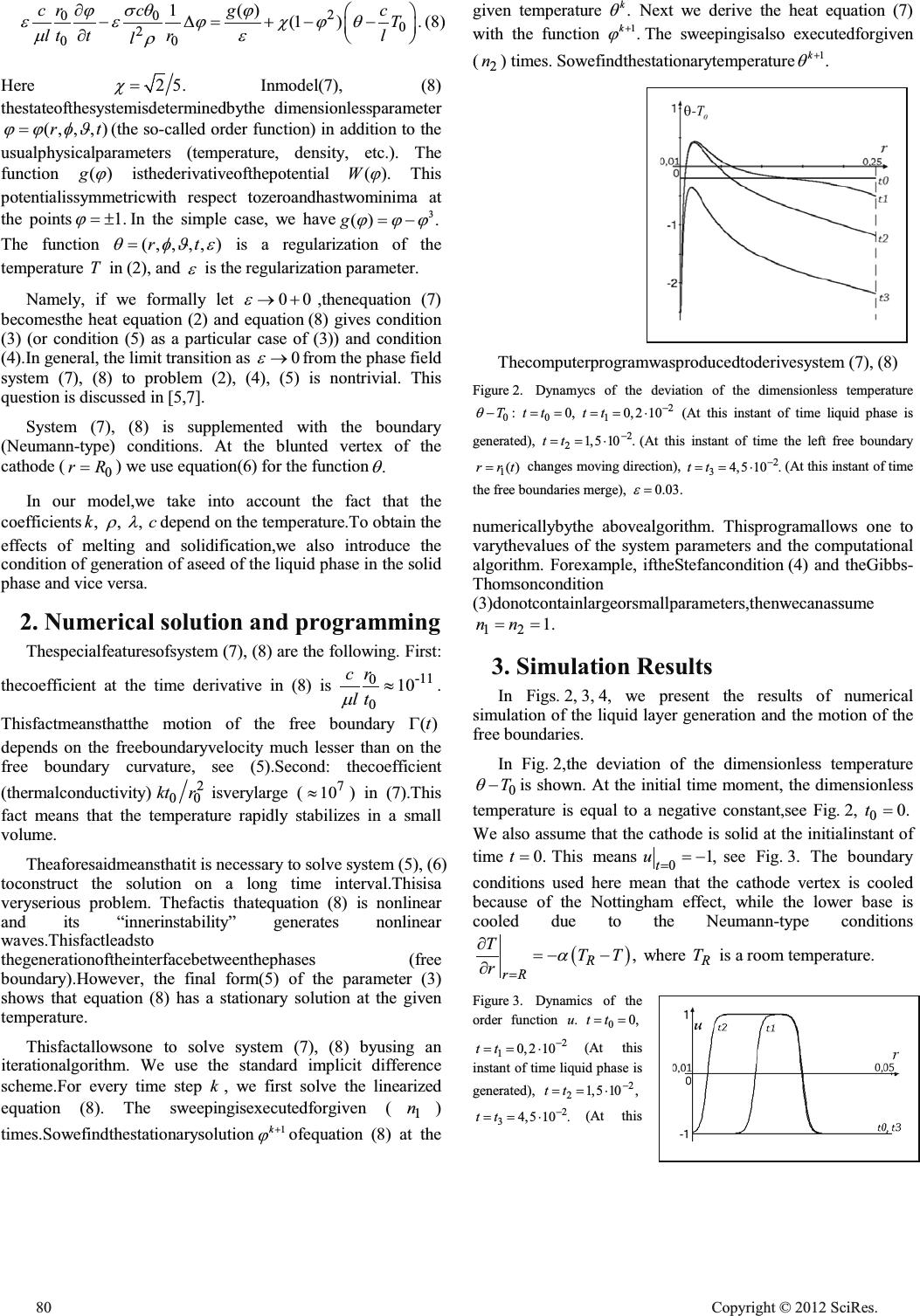 2 00 0 2 00 1() (1 ). rc cgc T lt trl l VT MM HHMFMT PH U w§· ' ¨¸ w©¹ Here 25. F Inmodel(7), (8) thestateofthesystemisdeterminedbythe dimensionlessparameter (, ,,)rt MMI- (the so-called order function) in addition to the usualphysicalparameters (temperature, density, etc.). The function ()g M isthederivativeofthepotential ().W M This potentialissymmetricwith respect tozeroandhastwominima at the points 1. M r In the simple case, we have 3 () .g MMM The function (, ,,, )rt TI-H is a regularization of the temperature T in (2), and H is theregularizationparameter. Namely, if we formally let 00 H o,thenequation (7) becomesthe heat equation (2) and equation(8) gives condition (3) (or condition (5) as a particular case of (3)) and condition (4).In general, the limit transition as 0 H o from the phase field system (7), (8) to problem (2), (4), (5) is nontrivial. This question is discussed in [5,7]. System (7), (8) is supplemented with the boundary (Neumann-type) conditions. At the blunted vertex of the cathode ( 0 rR ) we use equation(6) for the function . T In our model,we take into account the fact that the coefficients ,k , U , O c depend on the temperature.To obtain the effects of melting and solidification,we also introduce the condition of generation of aseed of the liquid phase in the solid phase and vice versa. 2. Numerical solution and programming Thespecialfeaturesofsystem (7), (8) are the following.First: thecoefficient at the time derivative in (8) is -11 0 0 10 r c lt P | . Thisfactmeansthatthe motion of the free boundary ()t* depends on the freeboundaryvelocity much lesser than on the free boundary curvature, see (5).Second: thecoefficient (thermalconductivity) 2 00 kt r isverylarge ( 7 10| ) in (7).This fact means that the temperature rapidly stabilizes in a small volume. Theaforesaidmeansthatit is necessary to solve system(5), (6) toconstruct the solution on a long time interval.Thisisa veryserious problem. Thefactis thatequation (8) is nonlinear and its “innerinstability” generates nonlinear waves.Thisfactleadsto thegenerationoftheinterfacebetweenthephases(free boundary).However, the final form(5) of the parameter (3) shows that equation (8) has a stationary solutionat the given temperature. Thisfactallowsone to solvesystem (7), (8) byusing an iterationalgorithm. We use the standard implicit difference scheme.For every time step k , we first solve the linearized equation (8). The sweepingisexecutedforgiven ( 1 n ) times.Sowefindthestationarysolution 1k M ofequation (8) at the given temperature . k T Next we derive the heat equation (7) with the function 1. k M The sweepingisalso executedforgiven ( 2 n ) times. Sowefindthestationarytemperature 1 . k T Thecomputerprogramwasproducedtoderivesystem(7), (8) Figure 2. Dynamycs of the deviation of the dimensionless temperature 0 :T T 0 0,tt 2 1 0, 210tt (At this instant of time liquid phase is generated), 2 21, 510.tt (At this instant of time the left free boundary 1 ()rrt changes moving direction), 2 3 4,5 10.tt (At this instant of time the free boundaries merge), 0.03. H numericallybythe abovealgorithm. Thisprogramallows one to varythevalues of the system parametersand the computational algorithm. Forexample, iftheStefancondition(4) and theGibbs- Thomsoncondition (3)donotcontainlargeorsmallparameters,thenwecanassume 12 1.nn 3. Simulation Results In Figs. 2, 3, 4, we present the results of numerical simulation of the liquid layer generation and the motion of the free boundaries. In Fig. 2,the deviation of the dimensionless temperature 0 T T is shown. At the initial time moment, the dimensionless temperature is equal to a negative constant,see Fig.2, 0 0.t We also assume that the cathode is solid at the initialinstant of time 0.t This means 0 1, t u see Fig.3. The boundary conditions used here mean that the cathode vertex is cooled because of the Nottingham effect, while the lower base is cooled due to the Neumann-type conditions , R rR TTT r D w w where R T is a room temperature. Figure 3. Dynamics of the order function .u 0 0,tt 2 10, 210tt (At this instant of time liquid phase is generated), 2 2 1, 510,tt 2 3 4,5 10.tt (At this 80 Cop y ri g ht © 2012 SciRes. 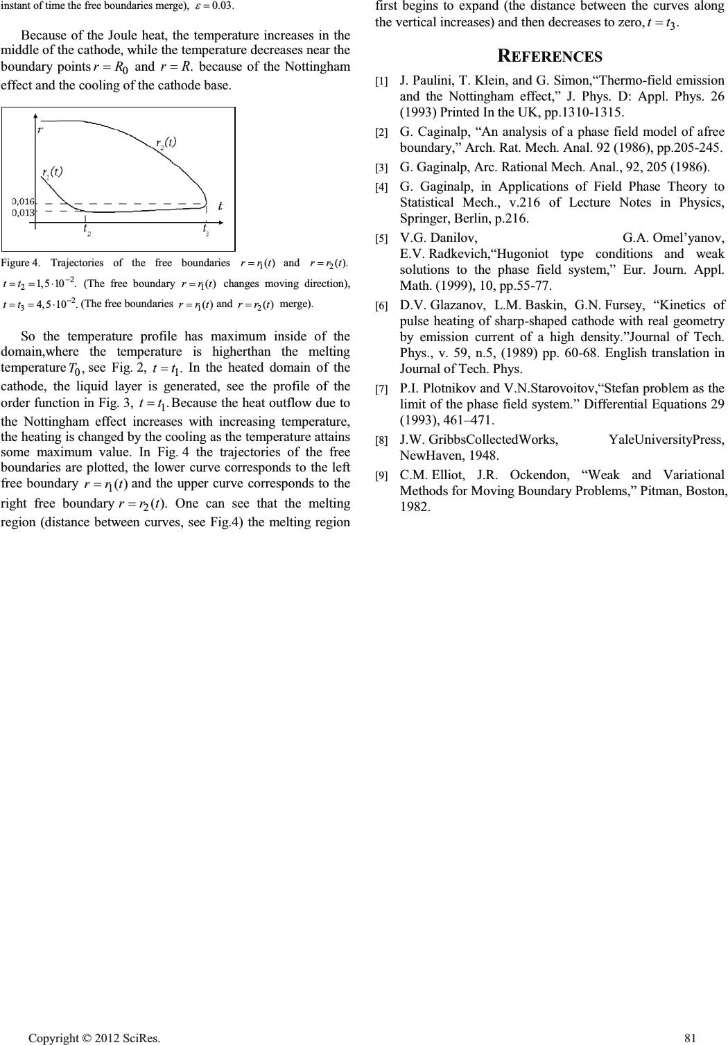 instant of time the free boundaries merge), 0.03. H Because of the Joule heat, the temperature increases in the middle of the cathode, while the temperaturedecreases near the boundary points 0 rR and .rR because of the Nottingham effect and the cooling of the cathode base. Figure 4. Trajectories of the free boundaries 1()rrt and 2().rrt 2 21, 510.tt (The free boundary 1 ()rrt changes moving direction), 2 3 4,5 10.tt (The free boundaries 1 ()rrt and 2 ()rrt merge). So the temperature profile has maximum inside of the domain,where the temperature is higherthan the melting temperature 0,T see Fig.2, 1.tt In the heated domain of the cathode, the liquid layer is generated, see the profile of the order function in Fig.3, 1.tt Because the heat outflow due to the Nottingham effect increases with increasing temperature, the heating is changed by the cooling as the temperature attains some maximum value. In Fig.4 the trajectories of the free boundaries are plotted, the lower curve corresponds to the left free boundary 1()rrt and the upper curve corresponds to the right free boundary2().rrt One can see that the melting region (distance between curves, see Fig.4) the melting region first begins to expand (the distance between the curves along the vertical increases) and then decreases to zero, 3.tt REFERENCES [1] J. Paulini, T. Klein, and G. Simon,“Thermo-field emission and the Nottingham effect,” J. Phys. D: Appl. Phys. 26 (1993) Printed In the UK, pp.1310-1315. [2] G. Caginalp, “An analysis of a phase field model of afree boundary,” Arch. Rat. Mech. Anal. 92 (1986), pp.205-245. [3] G. Gaginalp, Arc. Rational Mech. Anal., 92, 205 (1986). [4] G. Gaginalp, in Applications of Field Phase Theory to Statistical Mech., v.216 of Lecture Notes in Physics, Springer, Berlin, p.216. [5] V.G.Danilov, G.A.Omel’yanov, E.V.Radkevich,“Hugoniot type conditions and weak solutions to the phase field system,” Eur. Journ. Appl. Math. (1999), 10, pp.55-77. [6] D.V. Glazanov,L.M. Baskin,G.N. Fursey,“Kinetics of pulse heating of sharp-shaped cathode with real geometry by emission current of a high density.”Journal of Tech. Phys., v. 59, n.5, (1989) pp. 60-68. English translation in Journal of Tech. Phys. [7] P.I. Plotnikov and V.N.Starovoitov,“Stefan problem as the limit of the phase field system.” Differential Equations 29 (1993), 461–471. [8] J.W. GribbsCollectedWorks, YaleUniversityPress, NewHaven, 1948. [9] C.M.Elliot, J.R. Ockendon, “Weak and Variational Methods for Moving Boundary Problems,” Pitman, Boston, 1982. Cop y ri g ht © 2012 SciRes.81 |