Applied Mathematics, 2010, 1, 215-221
doi:10.4236/am.2010.13026 Published Online September 2010 (http://www.SciRP.org/journal/am)
A Pest Management Epidemic Model with Time Delay and
Stage-Structure
Yumin Ding1, Shujing Gao1, Yujiang Liu1, Yun Lan2
1Key Laboratory of Jiangxi Province for Numerical Simulation and Emulation Techniques,
Gannan Normal University, Ganzhou, China
2Jiangxi Environmental Engineering Vocational College, Ganzhou, China
Received June 12, 2010; revised July 22, 2010; accepted July 25, 2010
Abstract
In this paper, an SI epidemic model with stage structure is investigated. In this model, impulsive biological
control which release infected pest to the field at a fixed time periodically is considered, and obtained the
sufficient conditions for the global attractivity of pest-extinction periodic solution and permanence of the
system. We also prove that all solutions of the model are uniformly ultimately bounded. The sensitive analy-
sis on the two thresholds and to the changes of the releasing amounts of infected pest is shown by numerical
simulations. Our results provide a reliable tactic basis for the practice of pest management.
Keywords: Pest Management, Stage Structure, Impulsive System, Permanence
1. Introduction
Pests outbreak often cause serious ecological and eco-
nomic problems, and the warfare between human and
pests has sustained for thousands of years. With the de-
velopment of society and the progress of science and
technology, a great deal of pesticides were used to control
pests, because they can quickly kill a significant portion of
pest population and sometimes provide the only feasible
method for preventing economic loss. However, pesticide
pollution is also recognized as a major health hazard to
human beings and beneficial insects. At present, more and
more people are concerned about the effects of pesticide
residues on human health and on the environment [1].
In natural world, there are many insects whose indi-
vidual members have a life history that takes them
through two stages, larva and mature. Pathogens may not
be effective against laver, that is, the disease only attacks
the susceptible mature pest population. For example,
saltcedar leaf beetle is such a pest. Pest control strategies
have been attracted many experts over the past years.
Recently, stage-structured models have received much
attraction [2,3]. However, the epidemic models with
stage-structure have been seldom studied. Zhang et al. [4]
introduced the pest based on the stage-structure model
which incorporates a discrete delay and pulses in order to
investigate how epidemics influence the pest control
process. An SI model with impulsive perturbations on
diseased pest and spraying pesticides at fixed moment is
proposed and investigated in [5], which obtained the suf-
ficient conditions of the global attractivity of pest-ex-
tinction periodic solution and permanence of the system.
Incidence plays a very important role in research of
epidemic models, bilinear and standard incidence rates
have been frequently used in classical epidemic models
[6]. Several different incidence rates have been proposed
by researchers. Anderson et al. pointed out that standard
incidence is more suitable than bilinear incidence [7,8].
Levin et al. have adopted the incidence form like
qp
SI  or qp SI
N
 [9]. Lindstrom pointed out the crow-
ed incidence 2
() (1()()
)
StaStbS t   [10]. However
there are seldom authors have concerned the stage-
structured models under the simultaneous effect of dis-
ease and crowed incidence. A stage-structure model with
the crowed incident rate is considered in [11]. According
to the facts of pest management, we take the crowded
effect as the incidence rate. Therefore, in this paper, a
pest management epidemic model which with time delay
and stage-structure is considered.
The present paper is organized as follows. In the next
section, we formulate the pest management model. In
Section 3, some essential lemmas which will be used to
prove our main results are introduced. In Section 4,
global attractivity of the susceptible pest-eradication pe-

Y. M. DING ET AL.
216
riodic solution and the permanence of the model is ana-
lyzed. In the final section, we present some numerical
simulations to illustrate the results and point out some
future research directions.
2. Model Formulation
In this paper, we study the pest management epidemic
model:
2
2
()( ()) ()()( ()) (),
() ()
()(())()(), ,
1() ()
() ()
() (),
1() ()
()()(), , ,
L tBStStLteBStSt
StIt
S teBStStSttnT
aS tbSt
StIt
It dIt
aS tbSt
ItItIttnTnZ




 











 




  


 

(1)
with initial conditions
123 3
0
122
((),(),()) for [,0], (0)0, 1,2,3,
(0)(())( ),
i
r
tttC ti
eB d


 



 



 (2)
where all the coefficients of model (1) are nonnegative
and (),(),()LtStIt represent the larva, mature susceptible
and infected pest population at time t, respectively. The
model is derived from the following assumptions.
(H1) The death rate of larva population is proportional
to the existing larva population with proportionality con-
stant

, the death rate of mature susceptible and infected
pest population is proportional to the existing mature
susceptible and infected pest population with proportion-
ality constants

and d, respectively.
(H2) Only the susceptible pest population can repro-
duce. ()BSis a birth rate function of the susceptible pest
population for(0, )Swith ()BSis monotonically
decreasing, lim( )()
SBS B   exists and (0 )B


()B  , where 1min{ ,,}
2d
 .
(H3)

represents a constant time to maturity, the pro-
duct term(( ))( )eBStSt





describes that immature
pest who were laid at timet


and survive at time t.
(H4) The incident rate is the crowded effect.
2
()
1() ()
St
aS tbSt

 .
(H5)

is the releasing amounts of infected pest at
,1,2,,tnTn

 and T is the period of the impulsive
effect.
Before going into any detail, we simplify model (1)
and restrict our attention to the following model:
2
2
() ()
()( ()) ()(),
1() (),
() ()
() (),
1() ()
(), .
StIt
S teBStStSt
aS tbSttnT
StIt
It dIt
aS tbSt
Itt nT


 




 

 





 

 

(3)
The initial conditions for (3) are
2
23
((),())([,0],),(0)>0, 2,3.
i
ttCC Ri  


 (4)
3. Some Useful Lemmas
The solution of system (1), denoted by ()( (),
x
tLt

(), ())
T
St It is a piecewise continuous function
3
:,
x
RR

()
x
tis continuous on (,(1)),nT nT

nZ

and ()lim()
tnT
x
nTx t



exists. Before demonstra-
ting the main results, we need to give some lemmas
which will be used as follows.
Lemma 1. (see [11]). Let 123 ((),(), ()) 0ttt

 for
0.t


 Then any solution of system (1) is strictly
positive.
Lemma 2. Let the function [,]mPCRR

  satisfies
the inequalities
0
()()()(), ,, 1,2,,
()() ,,
k
kkkkk
mtptmtqtt ttt k
mtdmtb tt









where , [,]pqPCR R

 and0,
k
dk
b are constants.
Then

Y. M. DING ET AL.
217

0
0
0
0
0
0
0
()()exp(( ))
exp(())
exp()(), .
k
kkj
k
t
kt
ttt
t
jk
t
tttttt
tt
k
ts
stt
mt mtdpsds
dpsdsb
dpdqsdstt


 











The proof of this lemma is given in [12].
We now show that all solutions of (1) are uniformly
ultimately bounded.
Lemma 3. Any solution (( ),( ),( ))Lt St It of system
(1) is uniformly ultimately bounded. That is, there exists
a constant 0
1
T
T
e
Me




 
 such that () ,LtM

S(), I()tMtM for sufficiently large t.
Proof. Define ()()() ().VtLt StIt By simple
computation when,tnTwe calculate the derivative of
V along the solution of system (1)
()()() 2(),DVtBSSLS dIBSSLSI  

for (,( 1)).tnTn T
Then we derive
()(), (,(1)). DVtVBSSStnT nT 

Obviously, from conditions (H1) and (H2), we are easy
to know that there exists a constant 0

such that
(), (,(1)),DV tVtnTnT 
 
for n large enough.
When tnT, we get
()().VnT VnT


According to Lemma 2, we derive
()( )
00
() (0)
as .
1
t
tts tnT
nT t
T
T
Vt Veedse
eMt
e
 





 

 
 




Therefore by the definition of ()Vt , we obtain that
each positive solution of system (1) is uniformly ulti-
mately bounded. This completes the proof.
Lemma 4. Consider the following delay differential
equation:
12
()( )().
x
taxt axt

 (5)
where a1, a2 and

are all positive constants and
() 0xt  for [,0].t

 We have:
1) If 12 ,aa then lim()0 ;
xxt  
2) If 12 ,aa then lim( ).
xxt  
The proof of this lemma is given in [13].
Lemma 5 (see [11]). Consider the following impul-
sive system:
()(), ,
()(),,1,2,,
vtdv ttnT
vnTvnTt nTn 

 

 
 (6)
where , 0.d

 Then there exists a unique positive
periodic of system (6)
*()
(), (,(1)], ,
dt nT
vtvetnT nTnZ




which is globally asymptotically stable, where *
1dT
ve


.
4. Main Results
In this section that follows we determine the global at-
tractivity condition of the susceptible pest-extinction
periodic solution and the permanence of the system (3).
4.1. Global Attractivity of the Susceptible
Pest-Extinction Periodic Solution
Denote


2
*(0)(1)( 1)
dT
Be aMbMe
R





 
 (7)
where 1
T
T
e
Me






Theorem 1. Let((),())St Itbe any solution of system
(3), the susceptible pest-extinction periodic solution
(0,( ))
I
t
of (3) is globally attractive provided that
*1R

.
Proof. Since*1R

, we can choose 0

sufficiently
small such that
0
2
(0) 11
dT
dT
e
Be aM bMe











 

(8)
Note that () ()
I
tdIt

 , from Lemma 2 and Lemma
5, we have that for the given0

there exists an integer1 k
such that for (1)nT tnT

 ,1 nk
00
() ().
1
dT
dT
e
It Ite










 (9)
From condition (H1), (3) and (9), we yield
2
() (0)( )
(),
1
dS tBeSt
dt
St
aM bM










for 1
, .tnTnk

 

Y. M. DING ET AL.
218
Consider the following comparison differential system
2
() (0)( )
(),
1
dy tBeyt
dt
yt
aM bM










(10)
for 1
, tnT nk

 .
From (8), we have2
(0) 1 Be aM bM





 .
According to Lemma 4, we havelim()0.
tyt  
By the comparison theorem, we have lim sup()
t
St


lim( )0
tyt  . Incorporating into the positivity of()St ,
we know that
lim( )0
tSt 

Therefore, for any 10

 (sufficiently small), there
exists an integer 22 1
()kkTkT

 such that 1 ()St


for all 2 tkT.
Form system (3) and Lemma 5, we have
1
()
()() ()
dI t
dI tdIt
dt
  .
Then we have 12 () ()()ztItz t and 1() (),zt It
2() ()zt It as,twhile 1()ztand2()ztare the solu-
tions of
11
11
1
()(), ,
()(),,
(0 )(0 ),
ztdztt nT
ztztt nT
zI



 

 



and
212
22
2
()() (),,
()(), ,
(0 )(0 ),
ztdzttnT
ztztt nT
zI




 

 



respectively, 1
2
1
exp(()( ))
() 1exp(())
dtnT
zt dT


 

 for nT
(1)tnT . Therefore, for any20,

 there exists an
integer 3,k3 nksuch that
222
()() ()ItItz t

  
. for tnT.
Let 20

, we get 2() ()zt It
 Hence ()()
I
tIt
as t. This completes the proof.
4.2. Permanence
Persistence (or permanence) is an important property of
dynamical systems, in this section, we focus on the per-
manence of system (3).
Denote
*
()
*
((0) )(1)
.
SdT
Bee
R
 




 (11)
where *11 ln 10.
(0)
Sd
TBe







 





Theorem 2. Suppose *1R. Then there is a positive
constant qsuch that each positive solution ((),())StIt
of (3) satisfies ()St q, for sufficiently large t.
Proof. Let ((),())St It be the solution of system (3)
with initial condition (4). Note that the first equation of
(3) can be rewritten as
2
()() ()
( ()) ()()1()
(())().
t
t
dS tS tI t
eBSt StSt
dt aSbS t
d
eBSSd
dt












In the following we define:
()()(( ))( )
t
t
WtSt eBSS d







.
Then the derivative of ()Wt with respect to the solu-
tion of system (3) is governed by
2
()
(()) ()
1() ()
dWI t
eBSt St
dt aS tbSt









.
Since *1R, we can choose sufficiently small
*()
d
S

 and

such that
*
*
()
() 0
1SdT
eBS
e












. (12)
We claim that for any 00t, it is impossible that
*
()StS

for all0 tt. Suppose that the claim is not
valid. Then there is a 00t such that * ()St S for all
0
tt. It follows from the second equation of system (3)
that for
*
2
()() ()()()()
1() ()
dI tStI tdI tdSI t
dtaStbSt

 

Consider the comparison impulsive system for0 tt,
*
()() (),,
()(), ,
ztdS zttnT
ztztt nT



 




(13)
According to Lemma 1, we get the unique positive pe-
riodic solution of system (13)
*
*()( )
(), (1),
SdtnT
ztzenT tnT
 


is globally asymptotically stable, where *
*
()
1SdT
z
e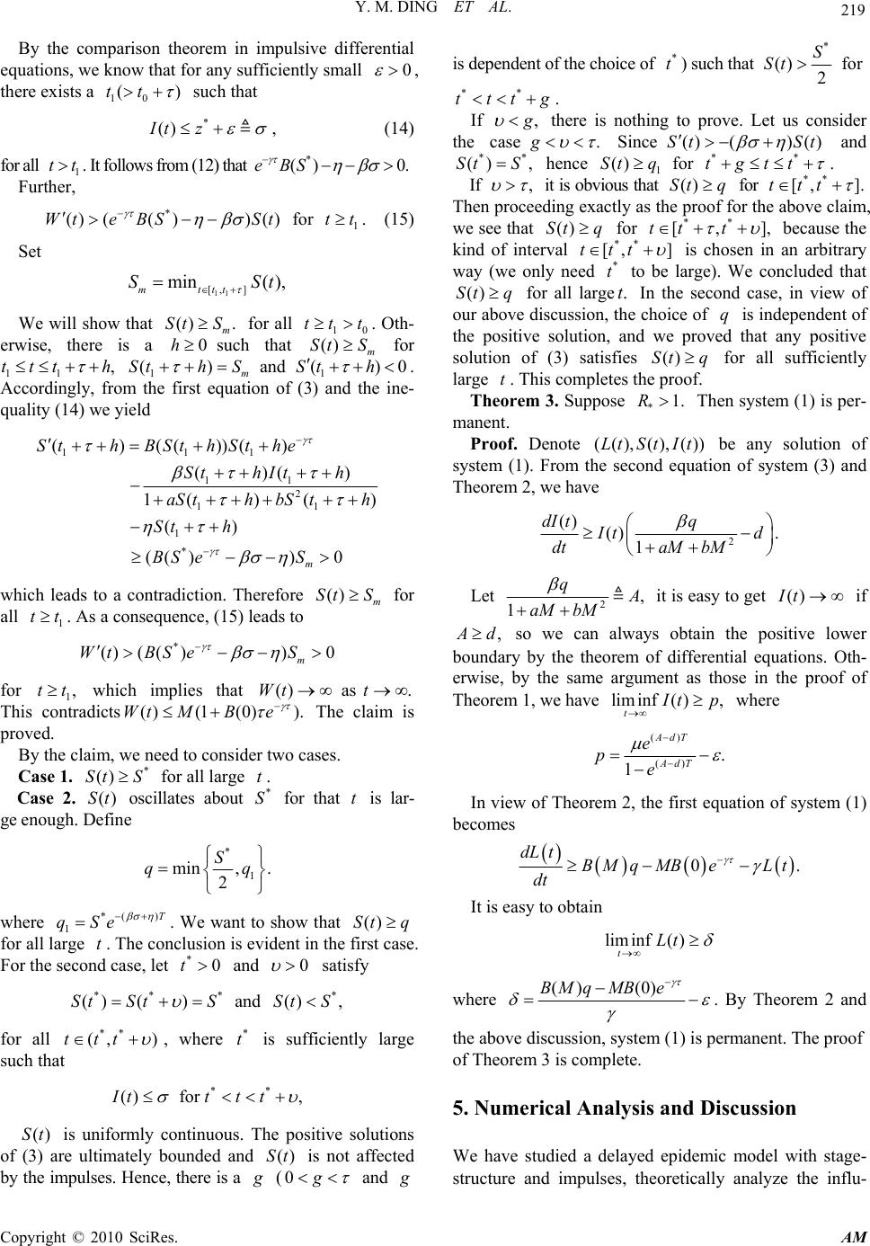



.

Y. M. DING ET AL.
219
By the comparison theorem in impulsive differential
equations, we know that for any sufficiently small 0

,
there exists a 10
()tt

 such that
*
()Itz

 , (14)
for all 1 tt. It follows from (12) that * () 0eBS


 .
Further,
*
()(())()Wte BSSt




for 1 tt. (15)
Set
11
[, ]
min( ),
mttt
SSt
 

We will show that () .
m
St S for all 10 tt t. Oth-
erwise, there is a 0hsuch that ()m St S for
11 ,ttth

  1
()
m
SthS

  and 1
()0Sth

 .
Accordingly, from the first equation of (3) and the ine-
quality (14) we yield
111
11
2
11
1
*
()(())()
()()
1( )( )
()
(())0
m
SthBSt hSthe
St hIt h
aSthbSth
St h
BS eS






 


 
 



which leads to a contradiction. Therefore () m
St S for
all 1 tt. As a consequence, (15) leads to
*
()( ())0
m
Wt BSeS

 


for 1,tt which implies that ()Wt as.t
This contradicts()(1(0) ).Wt MBe




 The claim is
proved.
By the claim, we need to consider two cases.
Case 1. * ()St S for all large t.
Case 2. ()St oscillates about * S for that t is lar-
ge enough. Define
*
1
min, .
2
S
qq



where *( )
1
T
qSe
  
. We want to show that ()St q
for all large t. The conclusion is evident in the first case.
For the second case, let *0t and 0

 satisfy
** *
() ()StStS   and * () ,StS
for all ** (, )ttt

, where * t is sufficiently large
such that
**
() for ,Ittt t

 
()St is uniformly continuous. The positive solutions
of (3) are ultimately bounded and ()St is not affected
by the impulses. Hence, there is a
g
(0g

 and
g
is dependent of the choice of *
t) such that
*
() 2
S
St  for
**
tttg

.
If ,
g


there is nothing to prove. Let us consider
the case.
g



 Since()() ()St St


  and
**
() ,St S hence 1 ()St q for ** tgtt

.
If ,

  it is obvious that ()St q for ** [, ].ttt


Then proceeding exactly as the proof for the above claim,
we see that ()Stq for ** [, ],tt t

  because the
kind of interval **
[, ]ttt


 is chosen in an arbitrary
way (we only need * t to be large). We concluded that
()St q for all large.t In the second case, in view of
our above discussion, the choice of q is independent of
the positive solution, and we proved that any positive
solution of (3) satisfies ()St q for all sufficiently
large t. This completes the proof.
Theorem 3. Suppose *1.R Then system (1) is per-
manent.
Proof. Denote ((),(),())Lt St It be any solution of
system (1). From the second equation of system (3) and
Theorem 2, we have
2
() () .
1
dI tq
I
td
dt aM bM






Let 2,
1
q
A
aM bM

  it is easy to get ()It if
,
A
d so we can always obtain the positive lower
boundary by the theorem of differential equations. Oth-
erwise, by the same argument as those in the proof of
Theorem 1, we have lim inf(),
t
I
tp
  where
()
() .
1
AdT
AdT
e
pe







In view of Theorem 2, the first equation of system (1)
becomes

 
0.
dL tBM qMBeLt
dt



 
It is easy to obtain
lim inf()
tLt

 
where () (0)BM qMBe







. By Theorem 2 and
the above discussion, system (1) is permanent. The proof
of Theorem 3 is complete.
5. Numerical Analysis and Discussion
We have studied a delayed epidemic model with stage-
structure and impulses, theoretically analyze the influ-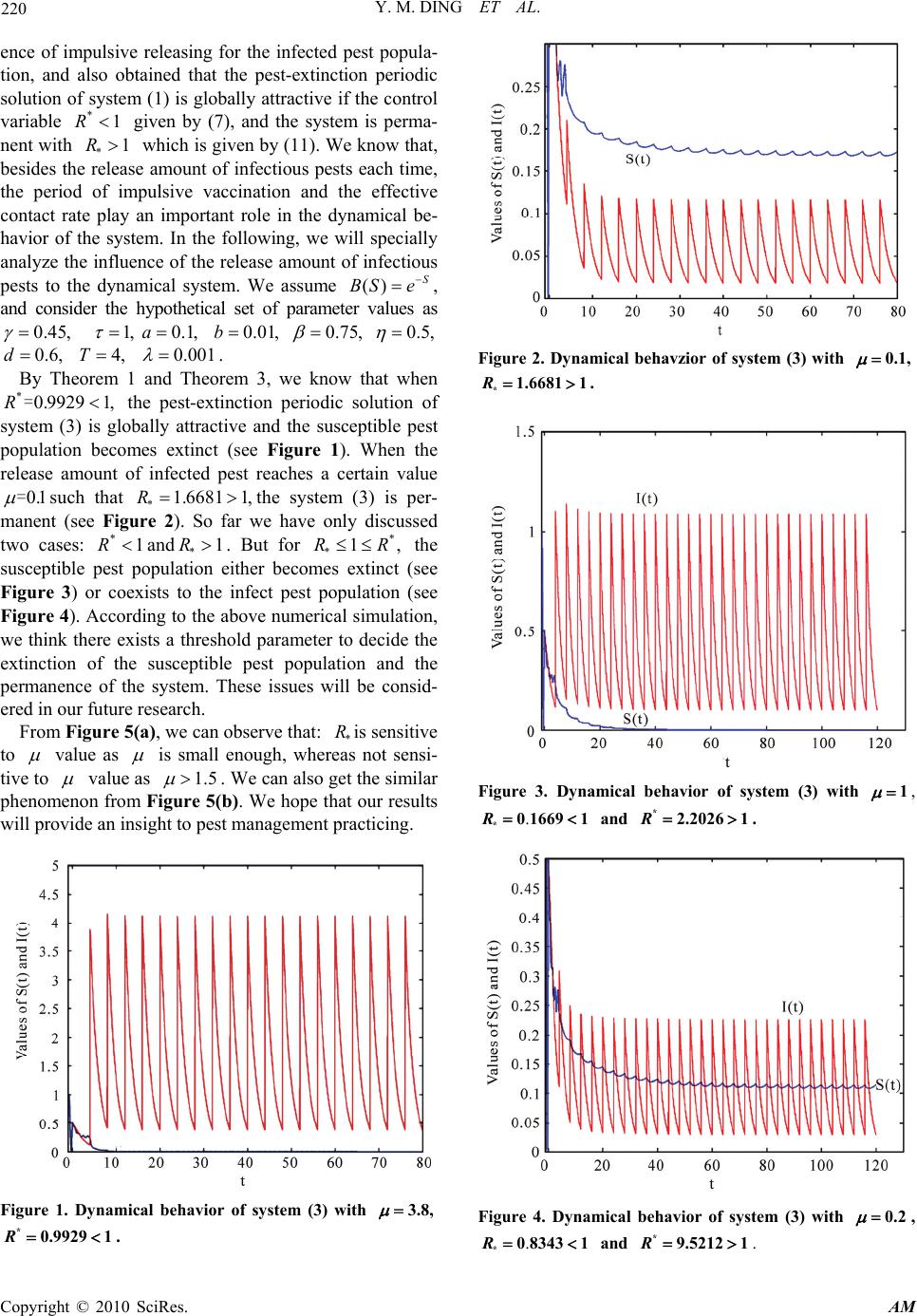

Y. M. DING ET AL.
220
ence of impulsive releasing for the infected pest popula-
tion, and also obtained that the pest-extinction periodic
solution of system (1) is globally attractive if the control
variable *1R given by (7), and the system is perma-
nent with *1R which is given by (11). We know that,
besides the release amount of infectious pests each time,
the period of impulsive vaccination and the effective
contact rate play an important role in the dynamical be-
havior of the system. In the following, we will specially
analyze the influence of the release amount of infectious
pests to the dynamical system. We assume ()S BSe

,
and consider the hypothetical set of parameter values as
0.45,

 1,

0.1,a 0.01,b

0.75,

 0.5,


0.6,d 4,T 0.001

.
By Theorem 1 and Theorem 3, we know that when
*0.9929 1,R= the pest-extinction periodic solution of
system (3) is globally attractive and the susceptible pest
population becomes extinct (see Figure 1). When the
release amount of infected pest reaches a certain value
0.1

=such that *1.6681 1,Rthe system (3) is per-
manent (see Figure 2). So far we have only discussed
two cases: *1Rand *1R. But for *
*1,RR the
susceptible pest population either becomes extinct (see
Figure 3) or coexists to the infect pest population (see
Figure 4). According to the above numerical simulation,
we think there exists a threshold parameter to decide the
extinction of the susceptible pest population and the
permanence of the system. These issues will be consid-
ered in our future research.
From Figure 5(a), we can observe that: *
Ris sensitive
to

value as

is small enough, whereas not sensi-
tive to

value as 1.5

. We can also get the similar
phenomenon from Figure 5(b). We hope that our results
will provide an insight to pest management practicing.
Figure 1. Dynamical behavior of system (3) with 3.8,


*0.9929 1R.
Figure 2. Dynamical behavzior of system (3) with 0.1,


*1.6681 1

R.
Figure 3. Dynamical behavior of system (3) with 1


,
.
*0 16691

R and *2.20261

R.
Figure 4. Dynamical behavior of system (3) with 0.2


,
.
*0 83431

R and *9.5212 1

R.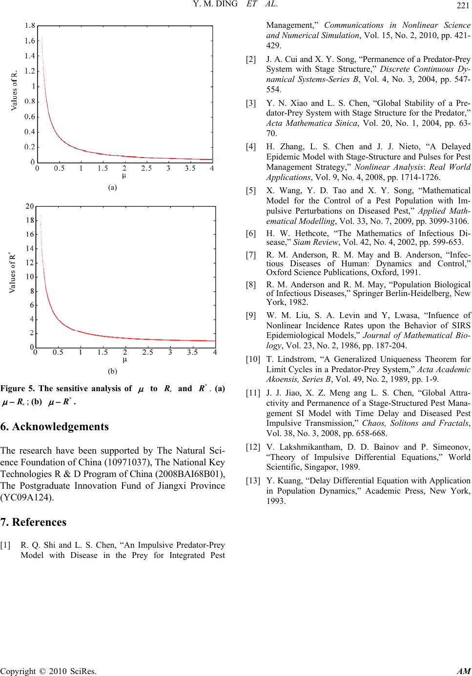

Y. M. DING ET AL.
221
(a)
(b)
Figure 5. The sensitive analysis of

to *
R
and *
R
. (a)
*


R
; (b) *


R
.
6. Acknowledgements
The research have been supported by The Natural Sci-
ence Foundation of China (10971037), The National Key
Technologies R & D Program of China (2008BAI68B01),
The Postgraduate Innovation Fund of Jiangxi Province
(YC09A124).
7. References
[1] R. Q. Shi and L. S. Chen, “An Impulsive Predator-Prey
Model with Disease in the Prey for Integrated Pest
Management,” Communications in Nonlinear Science
and Numerical Simulation, Vol. 15, No. 2, 2010, pp. 421-
429.
[2] J. A. Cui and X. Y. Song, “Permanence of a Predator-Prey
System with Stage Structure,” Discrete Continuous Dy-
namical Systems-Series B, Vol. 4, No. 3, 2004, pp. 547-
554.
[3] Y. N. Xiao and L. S. Chen, “Global Stability of a Pre-
dator-Prey System with Stage Structure for the Predator,”
Acta Mathematica Sinica, Vol. 20, No. 1, 2004, pp. 63-
70.
[4] H. Zhang, L. S. Chen and J. J. Nieto, “A Delayed
Epidemic Model with Stage-Structure and Pulses for Pest
Management Strategy,” Nonlinear Analysis: Real World
Applications, Vol. 9, No. 4, 2008, pp. 1714-1726.
[5] X. Wang, Y. D. Tao and X. Y. Song, “Mathematical
Model for the Control of a Pest Population with Im-
pulsive Perturbations on Diseased Pest,” Applied Math-
ematical Modelling, Vol. 33, No. 7, 2009, pp. 3099-3106.
[6] H. W. Hethcote, “The Mathematics of Infectious Di-
sease,” Siam Review, Vol. 42, No. 4, 2002, pp. 599-653.
[7] R. M. Anderson, R. M. May and B. Anderson, “Infec-
tious Diseases of Human: Dynamics and Control,”
Oxford Science Publications, Oxford, 1991.
[8] R. M. Anderson and R. M. May, “Population Biological
of Infectious Diseases,” Springer Berlin-Heidelberg, New
York, 1982.
[9] W. M. Liu, S. A. Levin and Y, Lwasa, “Infuence of
Nonlinear Incidence Rates upon the Behavior of SIRS
Epidemiological Models,” Journal of Mathematical Bio-
logy, Vol. 23, No. 2, 1986, pp. 187-204.
[10] T. Lindstrom, “A Generalized Uniqueness Theorem for
Limit Cycles in a Predator-Prey System,” Acta Academic
Akoensis, Series B, Vol. 49, No. 2, 1989, pp. 1-9.
[11] J. J. Jiao, X. Z. Meng ang L. S. Chen, “Global Attra-
ctivity and Permanence of a Stage-Structured Pest Mana-
gement SI Model with Time Delay and Diseased Pest
Impulsive Transmission,” Chaos, Solitons and Fractals,
Vol. 38, No. 3, 2008, pp. 658-668.
[12] V. Lakshmikantham, D. D. Bainov and P. Simeonov,
“Theory of Impulsive Differential Equations,” World
Scientific, Singapor, 1989.
[13] Y. Kuang, “Delay Differential Equation with Application
in Population Dynamics,” Academic Press, New York,
1993.