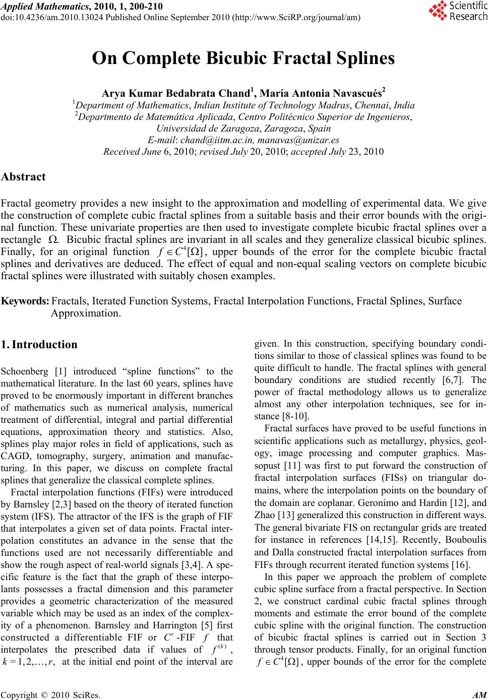Applied Mathematics, 2010, 1, 200-210
doi:10.4236/am.2010.13024 Published Online September 2010 (http://www.SciRP.org/journal/am)
On Complete Bicubic Fractal Splines
Arya Kumar Bedabrata Chand1, María Antonia Navascués2
1Department of Mathematics, Indian Institute of Technology Madras, Chennai, India
2Departmento de Matemática Aplicada, Centro Politécnico Superior de Ingenieros,
Universidad de Zaragoza, Zaragoza, Spain
Received June 6, 2010; revised July 20, 2010; accepted July 23, 2010
Abstract
Fractal geometry provides a new insight to the approximation and modelling of experimental data. We give
the construction of complete cubic fractal splines from a suitable basis and their error bounds with the origi-
nal function. These univariate properties are then used to investigate complete bicubic fractal splines over a
rectangle . Bicubic fractal splines are invariant in all scales and they generalize classical bicubic splines.
Finally, for an original function 4[]fC, upper bounds of the error for the complete bicubic fractal
splines and derivatives are deduced. The effect of equal and non-equal scaling vectors on complete bicubic
fractal splines were illustrated with suitably chosen examples.
Keywords: Fractals, Iterated Function Systems, Fractal Interpolation Functions, Fractal Splines, Surface
Approximation.
1. Introduction
Schoenberg [1] introduced “spline functions” to the
mathematical literature. In the last 60 years, splines have
proved to be enormously important in different branches
of mathematics such as numerical analysis, numerical
treatment of differential, integral and partial differential
equations, approximation theory and statistics. Also,
splines play major roles in field of applications, such as
CAGD, tomography, surgery, animation and manufac-
turing. In this paper, we discuss on complete fractal
splines that generalize the classical complete splines.
Fractal interpolation functions (FIFs) were introduced
by Barnsley [2,3] based on the theory of iterated function
system (IFS). The attractor of the IFS is the graph of FIF
that interpolates a given set of data points. Fractal inter-
polation constitutes an advance in the sense that the
functions used are not necessarily differentiable and
show the rough aspect of real-world signals [3,4]. A spe-
cific feature is the fact that the graph of these interpo-
lants possesses a fractal dimension and this parameter
provides a geometric characterization of the measured
variable which may be used as an index of the complex-
ity of a phenomenon. Barnsley and Harrington [5] first
constructed a differentiable FIF or r C-FIF
f
that
interpolates the prescribed data if values of ()k
f
,
=1,2,, ,kr at the initial end point of the interval are
given. In this construction, specifying boundary condi-
tions similar to those of classical splines was found to be
quite difficult to handle. The fractal splines with general
boundary conditions are studied recently [6,7]. The
power of fractal methodology allows us to generalize
almost any other interpolation techniques, see for in-
stance [8-10].
Fractal surfaces have proved to be useful functions in
scientific applications such as metallurgy, physics, geol-
ogy, image processing and computer graphics. Mas-
sopust [11] was first to put forward the construction of
fractal interpolation surfaces (FISs) on triangular do-
mains, where the interpolation points on the boundary of
the domain are coplanar. Geronimo and Hardin [12], and
Zhao [13] generalized this construction in different ways.
The general bivariate FIS on rectangular grids are treated
for instance in references [14,15]. Recently, Bouboulis
and Dalla constructed fractal interpolation surfaces from
FIFs through recurrent iterated function systems [16].
In this paper we approach the problem of complete
cubic spline surface from a fractal perspective. In Section
2, we construct cardinal cubic fractal splines through
moments and estimate the error bound of the complete
cubic spline with the original function. The construction
of bicubic fractal splines is carried out in Section 3
through tensor products. Finally, for an original function
4[]fC

, upper bounds of the error for the complete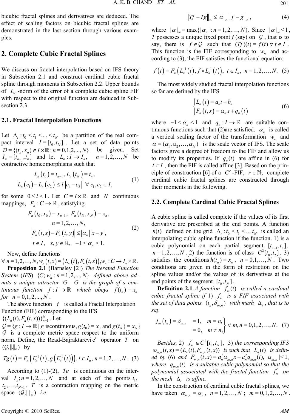

A. K. B. CHAND ET AL.
201
bicubic fractal splines and derivatives are deduced. The
effect of scaling factors on bicubic fractal splines are
demonstrated in the last section through various exam-
ples.
2. Complete Cubic Fractal Splines
We discuss on fractal interpolation based on IFS theory
in Subsection 2.1 and construct cardinal cubic fractal
spline through moments in Subsection 2.2. Upper bounds
of L-norm of the error of a complete cubic spline FIF
with respect to the original function are deduced in Sub-
section 2.3.
2.1. Fractal Interpolation Functions
Let 01 :<< ... <
tN
tt t be a partition of the real com-
pact interval 0 =[ ,]
N
I
tt . Let a set of data points
}0,1,2,...,=:),{(= NnIxt nn  be given. Set
1
=[, ]
nnn
I
tt
 and let :, nn
LI I =1,2, ,nN be
contractive homeomorphisms such that



 
01
121212
=, =,
,,
nnnNn
nn
Ltt Ltt
LcLclccccI


(1)
for some 0<1l. Let =CI and N continuous
mappings, :
n
FC, satisfying



 
00 1
,= ,,=,
=1,2,,,
,, ,
,,, 1<<1.
nnnNNn
nn n
n
F
txxFt xx
nN
F
txF tyxy
tI xy







(2)
Now, define functions
  
=1,2,, ,,=,,,:
nnnnn
nNwtxLtFtxwCI


.
Proposition 2.1 (Barnsley [2]) The Iterated Function
System (IFS) {;:= 1, 2,...,}
n
CwnN defined above ad-
mits a unique attractor G. G is the graph of a con-
tinuous function :fI which obeys ()=
nn
f
tx
for =0,1, 2,...,nN.
The above function
f
is called a Fractal Interpolation
Function (FIF) corresponding to the IFS
=1
{((),( ,))}
N
nn n
LtFtx . Let
}=)(and=)(,usiscontinuo|:{=00NN xtgxtggIg 

is a complete metric space respect to the uniform
norm. Define, the Read-Bajraktarevic operator T on
).,(  by
 
 
11
=, ,,=1,2,,.
nn nn
TgtFL tgL tt InN

 (3)
According to (1)-(2), Tg is continuous on the inter-
val ;=1,2,,
n
I
nN and at each of the points1,t
21
,,
N
tt

. T is a contraction mapping on the metric
space ).,(
 i.e.
,Tf Tgfg 


  (4)
where ||=max{| |:=1,2,,}
nnN


. Since ||<1

,
T possesses a unique fixed point f (say) on

, that is to
say, there is 

f such that ()()=()Tftf ttI

.
This function is the FIF corresponding to n
w and ac-
cording to (3), the FIF satisfies the functional equation:








11
=, ,,=1,2,,.
nn nn
f
tFLtfLttInN


(5)
The most widely studied fractal interpolation functions
so far are defined by the IFS


 
=
,=
nnn
nnn
Lt atb
F
txx q t 




 (6)
where 1< <1
n


and :
n
qI are suitable con-
tinuous functions such that (2)are satisfied. n

is called
a vertical scaling factor of the transformation n w and
12
=( ,,,)
N

   is the scale vector of IFS. The scale
factors give a degree of freedom to the FIF and allow us
to modify its properties. If ()
n
qt are affine in (6) for
tI

, then the FIF is called affine [3]. Based on the prin-
ciple of construction [6] of a r
C-FIF, ,r complete
cardinal cubic fractal splines are constructed through
their moments in the following.
2.2. Complete Cardinal Cubic Fractal Splines
A cubic spline is called complete if the values of its first
derivative are prescribed at the end points. A function
()ht defined on the grid 01 :<<
tN
tt t

 is called an
interpolating cubic spline function if the function. 1) is a
cubic polynomial on each partial segment 1
[,],
nn
tt

=1,2, ,
nN..2) the function is of class 2
02
[, ]Ctt . 3)
satisfies the conditions()=
nn
htx , =0,1,,nN. Two
conditions are given in the form of restriction on the
spline values and/or the values of its derivatives at the
end points of the segment 0
[, ]
N
tt .
Definition 2.1 A function ()
m
f
t is called a cardinal
cubic fractal spline if 1) m
f
is a FIF associated with
the set of data points ,
(, )
nmn
t

with mesh t , that is to
say


,
==1,=,
,=0,1, 2,,.
=0, ,
mn mn
ftmn mn N
mn




 (7)
Besides, 2) 2
0
[, ],
mN
f
Ctt 3) the corresponding IFS
,,
(, )=((),(, ))
mnn mn
txLtFtx

is such that ()
n
Lt is defin-
ed by (6) and 22
,,,,
(, )=(),||<1
mnnmnn mnmn
Ftxa xaqt  ,
where ,()
mn
qt is a suitable cubic polynomial so that the
polynomial associated with the fractal function '
m
f

on
the mesh t

is affine.
In the construction of cardinal cubic fractal splines, we
have taken ,=
mn n

 , =1,2,,nN; =0,1,2,,mN.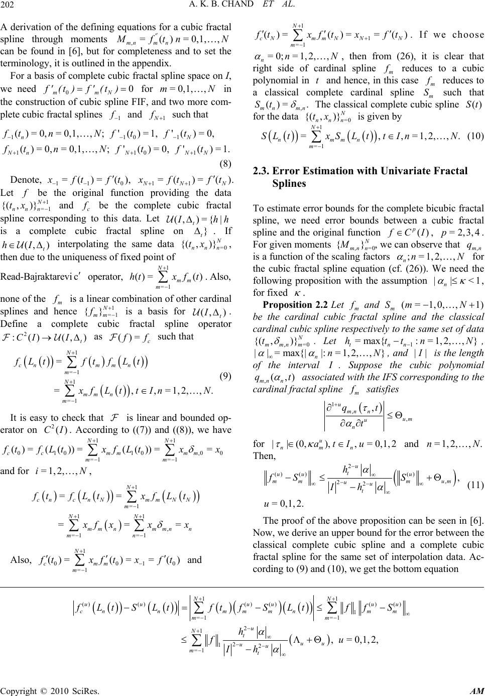

A. K. B. CHAND ET AL.
202
A derivation of the defining equations for a cubic fractal
spline through moments '
,=()=0,1,, mnm n
M
ftn N

can be found in [6], but for completeness and to set the
terminology, it is outlined in the appendix.
For a basis of complete cubic fractal spline space on I,
we need 00
mmN
f' (t )f' (t) for =0,1, ,mN in
the construction of cubic spline FIF, and two more com-
plete cubic fractal splines 1
f
 and 1N
f
 such that
1101
1101
() = 0,=0,1,,;'() =1,'() = 0,
() = 0,=0,1,,;'() = 0,'()=1.
nN
NnN NN
ft nNftft
ftnNftf t




(8)
Denote, 11 0
=()= ()
x
ftf t

, 11
=()= ()
N
NN
x
ftf t


.
Let
f
be the original function providing the data
1
=1
{( ,)}N
nnn
tx 
 and c
f
be the complete cubic fractal
spline corresponding to this data. Let hhI t|{=),( 

is a complete cubic fractal spline on }
t

. If
),( t Ih 

interpolating the same data =0 {( ,)}
N
nnn
tx ,
then due to the uniqueness of fixed point of
Read-Bajraktarevi c operator,
1
=1
()= ()
N
mm
m
htx ft


. Also,
none of the m f is a linear combination of other cardinal
splines and hence 1
=1
{}
N
mm
f
 is a basis for ),( t
I


.
Define a complete cubic fractal spline operator
),()(:2
t
IIC

 as c
ff=)( such that


 



1
=1
1
=1
=
=,,=1, 2,,.
N
cn mmn
m
N
mm n
m
fLtftfLt
x
fLt tInN







(9)
It is easy to check that  is linear and bounded op-
erator on 2()CI. According to ((7)) and ((8)), we have
11
01010 ,00
=1 =1
()=( ())=( ())==
NN
cc mm mm
mm
f
tfLtxfLtx x 



and for =1,2, ,iN,
    

1
=1
11
,
=1 =1
==
===
N
cncnNmmN N
m
NN
mm nmmnn
mn
f
tfLtxfLt
x
fxx x 






Also,
1
0010
=1
()=()== ()
N
cmm
m
f
txftxft




 and
1
1
=1
()=()==()
N
cNmmN NN
m
f
txftxft



 
. If we choose
=0;=1,2,,
nnN

, then from (26), it is clear that
right side of cardinal spline m
f
reduces to a cubic
polynomial in t and hence, in this case m
f
reduces to
a classical complete cardinal spline m S such that
,
()=.
mn mn
St

The classical complete cubic spline ()St
for the data =0 {( ,)}
N
nnn
tx is given by




1
=1
=,,=1, 2,,.
N
nmmn
m
SL txSL ttInN



 (10)
2.3. Error Estimation with Univariate Fractal
Splines
To estimate error bounds for the complete bicubic fractal
spline, we need error bounds between a cubic fractal
spline and the original function ()
p
f
CI, =2,3,4p.
For given moments ,=
0
{}
N
mn n
M, we can observe that ,mn q
is a function of the scaling factors ;=1,2, ,
nnN

 for
the cubic fractal spline equation (cf. (26)). We need the
following proposition with the assumption || <1
n



,
for fixed

.
Proposition 2.2 Let m
f
and m S (= 1,0,,1)mN
be the cardinal cubic fractal spline and the classical
cardinal cubic spline respectively to the same set of data
,=0
{( ,)}N
mmnm
t  . Let 1 =max{: =1,2,, }
tnn
httnN

,
||=max{| |:=1,2,,}
nnN


, and ||
I
is the length
of the interval
I
. Suppose the cubic polynomial
,(,) mn n
qt

associated with the IFS corresponding to the
cardinal fractal spline m
f
satisfies


1
,
,
,
u
mn n
um
u
n
qt
t





for ||(0, ),,=0,1,2
u
nmn
atIu   and =1,2,,.nN
Then,

2
()()()
,
22,
=0,1,2.
u
t
uu u
mmm um
uu
t
h
fS S
Ih
u







 
 (11)
The proof of the above proposition can be seen in [6].
Now, we derive an upper bound for the error between the
classical complete cubic spline and a complete cubic
fractal spline for the same set of interpolation data. Ac-
cording to (9) and (10), we get the bottom equation
    

 

11
()()()()()()
1
=1 =1
2
1
2 12
=1
,=0,1, 2,
NN
u uuuuu
cnnmm mnm m
mm
u
Nt
uu
uu
mt
fLtSLtftfSLtffS
h
fu
Ih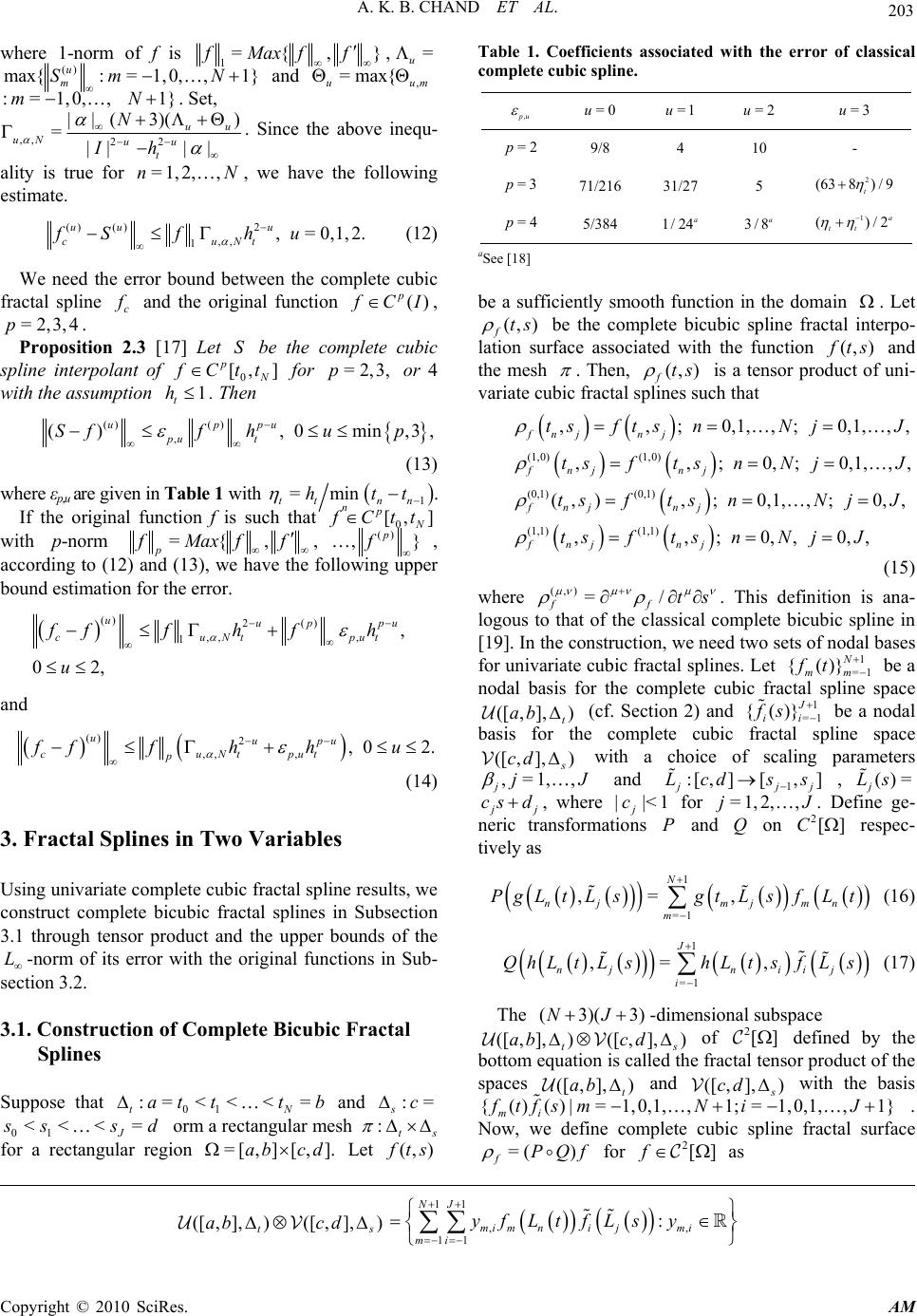









 





A. K. B. CHAND ET AL.
203
where 1-norm of f is 1={, }fMaxf f

,=
u

()
max{:=1, 0,,1}
u
m
Sm N
 and ,
=max{
uum

:=1,0,,m 1}N. Set,
,, 22
||( 3)()
=||| |
uu
uN uu
t
N
Ih







. Since the above inequ-
ality is true for =1,2,,nN , we have the following
estimate.
()()2
,,
1,=0,1, 2.
uu u
cuNt
fSfhu



 (12)
We need the error bound between the complete cubic
fractal spline c
f and the original function ()
p
f
CI,
=2,3,4p.
Proposition 2.3 [17] Let S be the complete cubic
spline interpolant of 0 [,]
p
N
f
Ctt for =2,3,p or 4
with the assumption 1
t
h. Then


()( )
,
(),0min,3,
uppu
pu t
Sff hup 



(13)
where εp,u are given in Table 1 with


1
=min
tt nn
n
htt


.
If the original function f is such that 0 [,]
p
N
f
Ctt
with p-norm ={, ,
p
fMaxff

()
,}
p
f

,
according to (12) and (13), we have the following upper
bound estimation for the error.

() 2()
,, ,
1,
02,
uup pu
cuNtput
fffh fh
u





 

and


() 2
,,, ,02.
uupu
cuNtput
p
fffh hu




 
(14)
3. Fractal Splines in Two Variables
Using univariate complete cubic fractal spline results, we
construct complete bicubic fractal splines in Subsection
3.1 through tensor product and the upper bounds of the
L-norm of its error with the original functions in Sub-
section 3.2.
3.1. Construction of Complete Bicubic Fractal
Splines
Suppose that 01 :=< <<=
tN
at ttb and :=
sc

01
<< <=
J
s
ssd orm a rectangular mesh :ts



for a rectangular region =[,][ ,].ab cd Let (, )
f
ts
Table 1. Coefficients associated with the error of classical
complete cubic spline.
,pu

=0u =1u =2u =3u
=2p 9/8 4 10 -
=3p 71/216 31/27 5 2 (638) / 9
t
 
=4 p 5/384 1/ 24a 3/8
a 1
()/2
a
tt



aSee [18]
be a sufficiently smooth function in the domain

. Let
(, )
fts

be the complete bicubic spline fractal interpo-
lation surface associated with the function (, )
f
ts and
the mesh

. Then, (, )
fts

is a tensor product of uni-
variate cubic fractal splines such that




 

 
(1,0) (1,0)
(0,1) (0,1)
(1,1) (1,1)
, ,;0,1,,;0,1,,,
,,;0,;0,1,,,
(,),;0,1,, ;0,,
,,;0,,0,,
fnj nj
fnj nj
fnj nj
fnj nj
tsftsnN jJ
tsftsnN jJ
tsftsnN jJ
tsftsnNjJ




 






(15)
where (,) =/
ff
ts

 



. This definition is ana-
logous to that of the classical complete bicubic spline in
[19]. In the construction, we need two sets of nodal bases
for univariate cubic fractal splines. Let 1
=1
{()}
N
mm
ft


be a
nodal basis for the complete cubic fractal spline space
)],,([t ba


(cf. Section 2) and 1
=1
{()}
J
ii
fs 

 be a nodal
basis for the complete cubic fractal spline space
)],,([ s dc

 with a choice of scaling parameters
,=1,,
jjJ

 and 1 :[ ,][,]
j
jj
Lcdss


,()=
j
Ls

j
j
csd

, where ||<1
j
c for =1,2, ,jJ. Define ge-
neric transformations P and Q on 2[]C respec-
tively as
 
 




1
=1
,= ,
N
nj mjmn
m
PgLtLsgtLsfLt




(16)
 






1
=1
,= ,
J
nj niij
i
QhLt L shLtsfL s




(17)
The (3)(3)NJ

-dimensional subspace
)],,([)],,([ st dcba





of ][
2

defined by the
bottom equation is called the fractal tensor product of the
spaces )],,([t
ba


and )],,([ s
dc  with the basis
{ ()()|=1,0,1, ,1;=1,0,1, ,1}
mi
ftfsmNiJ

 
.
Now, we define complete cubic spline fractal surface
=( )
fPQf

 for ][
2

f as
)],,([)],,([ st dcba  





11
,,
11
:
NJ
mi mnijmi
mi
yfLtfLs y

 






 

A. K. B. CHAND ET AL.
204
 


  


11
=1=1
,=,
,, ,
NJ
fn jmi
mi
mnij
LtLs fts
fLtfLs ts







(18)
where10 10 (,)= (,)/,(,)=(,)/
f
tsft stftsftss

 with
the analogues for 1 (,),
N
f
ts
 1
(, ),
J
fts
 11
(, )
f
ts

etc.
We now show that the function
f

satisfies the interpo-
lation conditions. According to (18), for {1, 2,,}nN
and {1, 2,,},jJ

 
 



 
11
=1=1
11
,,
=1=1
,= ,
=,
=,=,
fnjnNjJ
NJ
mimnij
mi
NJ
mimnijn j
mi
tsPQf LtLs
ftsftf s
f
ts fts











Similarly, 00 (, )= (,),=1,2,,
fj j
tsfts jJ

;
00
(, )= (, ),=1,2,,.
fn n
tsfts nN

 and 00 (, )=
fts

00
(, )
f
ts. Since 0 ()=( )=0
mmN
ftft
 for =0,1,,mN,
using (8), we have
11
(1,0) (1,0)
=1=1
(, )=(,)()()=(, )
NJ
f
njmimnij nj
mi
tsft sf tfsfts 



 ;
=0,;=0,1,, .nNj J Analogously, the rest of condi-
tions of definition (15) are true. Since, =
mm
f
S if
=0=1,2, ,
nnN

and =
ii
f
S
if=0=1,2, ,
jjJ

,
we can retrieve classical complete bicubic spline
f
S to
the original function
f
from (18).
3.2. Upper Bounds of L-Norm of Error
We will prove the L-norm error of complete bicubic
splines with the original function by using the following
notations analogous to those of Proposition 2.2 for the
t-variable.
Suppose ,ij q
; =1,2, ,jJ are cubic polynomials
associated with the IFSs for i
f
 such that
1
,
,
(,)
v
ij j
vi
v
j
qs
s





  for =1,0,1,,1iJ

,
*
||(0, )
v
j
j
c  
 with *
|| <1
j
  for fixed real *

.
Let, () =max{: =1,0,1,,1}
v
vi
Si J


 ,
,
=max{:=1,0,1,,1}
vvi
iJ 
  and
,, 22
||(3)()
=|| ||
vv
vJ vv
s
J
Jh









.
Suppose
4(,)
[]={::[],04}
uv
Cg gCuvand the
norm corresponding to this space is
(,)
4=max{ ;04}
uv
gguv
 .
Theorem 3.1 Let
f

be the complete bicubic fractal
spline to the original function 4[]fC. Then for an
arbitrary sequence of partitions,




(,) 24
,,4 ,
4
24
,,4 ,
24 24
,,4 ,,,4 ,,
0,2.
uv uuv
fuNtvut
vuv
vJs uvs
uuv vuv
uNtvutvJs uvs
ffhh
hh
hh hh
uv














 
 



Proof. In order to calculate the error, we will use the
generic transformations P and Q. Suppose that


   


 
=
ff
ffQffQfPf
fPf
 
 (19)
Consider


  


 



 
1
=1
,=,
,
nj nj
N
mj mn
m
f
PfL tL sfL tLs
ftLsfL t






For *
=
s
s fixed, (0, )* (())((),( ))
v
nj
PfL tLs
 is the
spline of (0,)* ((),())
v
nj
f
LtLs
 (with respect to the first
variable) and we can apply (14) for =4pv

since
(0, )*(4)
(.,())[ ,]
vv
j
f
LsC ab


. For 02u,





 
  

(,)
(,) **
(0, )*24
,,4 ,
4
24
,,4 ,
4
., .,
.,
uv
uv
jj
vuvu
juNtvut
v
uvu
uNtvut
fLsPf Ls
fLsh h
fh h












 

 (20)
Since the last term of (20) does not depend on *
s
,



(,)
(,)2 4
,,4 ,
4
uv
uvuvu
uNtvut
fPff hh





 (21)
In the same way,


(,) (,)24
,,4 ,
4
()
uvuvvu v
vJs uvs
fQff hh






(22)
Consider ()
f
Pf


and using their definitions,












 

 




 

11
=1 =1
1
11
=1
,
=, ,
=,= ,
fn j
NJ
mjmii jmn
mi
N
mjmnn j
m
PfLtLs
f
tLsftsfLsf Lt
RtLsfLtPRL tL s













 

where 1=().RfQf

Hence, we have
11
() (())=()
f
f
QfPfR PR


 . For * =
s
s fixed,
(0, )
1
()
v
PR is the cubic spline FIF of (0, )
1
v
R with respect
to the first variable and we can apply (14) taking
=4pv

.

A. K. B. CHAND ET AL.
205






(,)*(,)*
11
(0, )*24
1,,4,
4
.,().,( )
.,
uv uv
jj
vuvu
juNtvut
v
RLsPR Ls
RLsh h









 (23)
For 02v,









(0, )
(0, )*(0, )**
1.,= .,.,
v
vv
jj j
RLsf LsQfLs
 
and similarly to (22) for 02u,
  
(,) *24
1,,4,
4
.,
uvvu v
jvJsuvs
RLs fhh




 

and by (23), we get the first equation of the bottom ones.
The inequality of Theorem 3.1 follows from (21)-(24).
Remark. From Theorem 3.1, it can be observed that
the convergence of the bicubic fractal spline
f

is
slower than that of the case of the classical bicubic spline
f
S (see [20]). Since the classical bicubic spline is a
particular case of bicubic fractal spline, Theorem 3.1
generalizes the classical result. If there exist positive
reals k and l such that ,,
1
<
(
3
)
uN k
N

 and
,,
1
<
(
3
)
vJ l
J


, then the complete bicubic fractal spline
f

converges to the original function
f
in 2 C-norm
for uniform partitions.
4. Examples
First, we construct three different bases for complete
cubic fractal spline space with =[0,3]I, =3N and
three different sets of scaling vectors. These scaling vec-
tors play important role over classical splines in overall
shape of fractal approximants. The scaling vectors are
chosen for a basis of complete fractal splines as 1) Set I:
=0.9,= 1, 2,3
ni

; 2) Set II: =0.9,= 1, 2,3
ni

; 3)
Set III: 123
=0.5,= 0.9,= 0.7.

  In our examples,
12
111
()=,()=,
333
Lt tLt t
and 3
12
()= .
33
Lt t We com-
pute the moments ,mn M, =1,2,3n; =1,0, ,4m
from Equations (26)-(28). These values of moments for
three sets of bases are given in Table 2. These moments
are then used in IFS
2
{;(,)=((),(,)),= 1, 2,3}
nnn
wtxLtFxt n to compute
(,)
n
F
xt . From (5) and (25), we have the bottom equation.
where n
x
depends on the cardinal condition of the basis
elements m
f
, i.e., , =,=0,1, 2,3;=1,0,,4
nmn
xn m


.
Using the above IFS, we compute basis elements for
complete cubic fractal spline space with non-zero and
zero scaling vectors. When scaling factors are same in
Set I and Set II, the values of moments of 1
f
 and 4
f
;
0
f
and 3
f
; 1
f
and 2
f
follow a particular pattern
(see Table 2). This pattern is very close to the moments
pattern of classical complete cardinal splines (with zero
scale vector). That’s why pair-wise similarity between
complete cardinal fractal splines 1
f
 and 4
f
; 0
f
and
3
f
; 1
f
and 2
f
in such cases (see Figure 1(a) and
Figure 1(b)) observed as in classical complete cardinal
splines (see Figure 1(d)). But for unequal scaling factors
in Set III, there is no pattern between moments of com-
plete cardinal fractal splines and hence, their shapes are
completely different (see Figure 1(c)). The unequal
scaling factors provides an additional advantage of com-
plete cardinal fractal splines over their classical counter-
parts in smooth object modelling in engineering applica-
tions like computer graphics, CAD/CAM.
The non-zero scale vectors gives irregular shape to
fractal splines because '
n
f

are typical fractal functions,
i.e., fractal dimension of graph of '
n
f
 is non-integer.
These cardinal fractal splines differ from their classical
interpolants in the sense that they obey a functional rela-
tion related to self-similarity on smaller scales. Hence,
cardinal fractal splines are defined globally on the entire
domain. Moreover, classical complete splines are defined
piecewisely between consecutive nodes and hence, their
shapes can be defined locally. Importantly, if =0,
n

=1,2,3n, then we can retrieve the basis elements (see
Figure 1(d)) for the classical complete cubic spline
space. Using these three sets of vertical scaling vectors,
we have constructed complete bicubic splines in the fol-
lowing.
Some complete bicubic fractal splines are constructed
using the tensor product of univariate fractal splines for
the interpolation data given in Table 3. In all our examples,
we assume the same boundary conditions for complete





(,)
(,)2 424
11,,4, ,,4,
4.
uv
uvvuvuv u
vJs uvsuNtvut
RPRf hhhh





 
. (24)










3
3
,,3,1,0,,3
,1 ,0
10 3
3
1
,918 182
33
99,=1, 2,3,
233
mnn mmnn mmnn m
nn
mnnm
nn nn
M
Mt MMtMMt
Ftxx
MMt tt
xx xxn
 







 




 





A. K. B. CHAND ET AL.
206
Table 2. Moments for cardinal complete cubic fractal splines.
Basis Elements Moments Set I Set II Set III Classical Case
1,0
M −16.4058 −2.5546 −2.4586 −3.4667
1,1
M −10.7536 1.4714 0.6318 0.9333
1,2
M −12.5797 0.4584 −1.4137 −0.2667
1
f

1,3
M −10.9275 0.4844 −0.5122 0.1333
0,0
M
−24.4348 −2.8448 −2.7653 −4.4000
0,1
M
−14.5217 3.5448 2.0938 2.8000
0,2
M
−19.4783 0.3500 −2.2451 −0.8000
0
f
0,3
M
−15.5652 0.7396 −0.2621 0.4000
1,0
M
27.8261 3.3903 3.5365 5.6000
1,1
M
11.3913 −5.7266 −3.6048 −5.2000
1,2
M
22.6087 1.8319 3.6812 3.2000
1
f
1,3
M
12.1739 −1.2850 −2.0094 −1.6000
2,0
M
12.1739 −1.2850 −2.0094 −1.6000
2,1
M
22.6087 1.8319 1.3664 3.2000
2,2
M
11.3913 −5.7266 −1.0007 −5.2000
2
f
2,3
M
27.8261 3.3903 9.3235 5.6000
3,0
M
−15.5652 0.7396 1.2382 0.4000
3,1
M
−19.4783 0.3500 0.1447 −0.8000
3,2
M
−14.5217 3.5448 −0.4354 2.8000
3
f
3,3
M
−24.4348 −2.8448 −7.0520 −4.4000
4,0
M
10.9275 −0.4844 −0.7738 −0.1333
4,1
M
12.5797 −0.4584 −0.1938 0.2667
4,2
M
10.7536 −1.4714 1.0400 −0.9333
4
f
4,3
M
16.4058 2.5546 5.0306 3.4667
Table 3. Interpolation data for complete bicubic splines.
(, )
nj
f
ts 0=1s 1=2s 2=3s 3=3s
0=1t −1 11 −5 10
1=2t 2 14 3 15
2=3t 0 9 1 17
3=4t 1 10 3 13

A. K. B. CHAND ET AL.
207
(a) (b)
(c) (d)
Figure 1. Bases for complete cubic fractal spline space. (a) Cardinal cubic fractal splines with Set I; (b) Cardinal cubic fractal
splines with Set II; (c) Cardinal cubic fractal splines with Set III; (d) Classical cardinal cubic splines with =0,=1,2,3
nn

.
bicubic splines: (1,0) (,) = 5;= 0,3,= 0,1,2,3
nj
fts nj,
(0,1) (,)=3; =0,1,2,3, =0,3
nj
ftsnj, and(1,1)(,)=2
nj
fts;
=0,3j. The scaling vectors are same in both directions
in our first three examples, i.e., =
nj

for =nj
and we take these scale vectors as Set I, Set II and Set III
defined in above for univariate case. The cardinal splines
=
mi
f
f
 if =im in these cases for ,=1,0,,4.im 
Based on (18), the points of complete bicubic fractal
splines are generated and plotted in Figsures 2-4. The
effect of change in scaling factors from 0.9 to −0.9 on
complete bicubic spline can be seen from Figsures 2-3.
The difference in the shape of complete bicubic spline
for an unequal scaling factors can be observed by com-
paring Figure 4 with Figsures 2-3.
Next, we take scaling vectors in t-direction as Set I
and in s-direction as Set III and the corresponding com-
plete bicubic spline generated in Figure 5. It has similar-
ity with both Figure 2 and Figure 4 due to self-similar-
ity relation in t and s directions respectively. For Figure
6, we chose scaling vectors in t-direction as Set III and in
s-direction as Set II. The distinct deviation in s-direction
of complete bicubic spline is present in this case as in
Figure 3. Finally, we chose ==0
nj

,nj. Since
=
mm
fS and =
ii
f
S
 in this case, we retrieve the classical
complete bicubic spline
f
S in Figure 7. An infinite
number of complete bicubic splines can be constructed
interpolation the same data by choosing different sets of
scaling vectors. Hence, the presence of scaling vectors in
bicubic fractal splines provides an additional advantage
over classical bicubic splines in smooth surface model-
ling. Since bicubic fractal splines are invariant in all
scales, it can also be applied to bivariate image compres-
sion and zooming problems in image processing.
5. Conclusions
We introduced bases for complete cubic fractal splines
through cardinal fractal splines in the present work.
These cardinal fractal splines constructed through moments

A. K. B. CHAND ET AL.
208
Figure 2. Complete bicubic fractal spline with scale vectors
Set I in both directions.
Figure 3. Complete bicubic fractal spline with scale vectors
Set II in both directions.
Figure 4. Complete bicubic fractal spline with scale vectors
Set III in both directions.
Figure 5. Complete bicubic fractal spline with scale vectors
Set I, Set III.
Figure 6. Complete bicubic fractal spline with scale vectors
Set III, Set II.
Figure 7. Classical complete bicubic spline with zero scale
vector.

A. K. B. CHAND ET AL.
209
as in the classical case. Using tensor product of cardinal
cubic fractal splines, bicubic fractal splines introduced
over rectangular domains with rectangular partition.
These bicubic fractal splines are invariant in all scales
due to underlying fixed point equation. L-norm of the
error of complete cubic fractal spline with respect to the
original function []
p
fC , =2,3p or 4 has been
deduced. The presence of scaling factors can be ex-
ploited in bivariate optimization problems with pre-
scribed interpolation conditions. The effect of equal and
non-equal scaling factors in complete bicubic splines is
explained. The present work may play important role in
smooth surface modelling in computer graphics and im-
age processing applications.
6. Acknowledgements
The work was supported by the project No: SB 2005-
0199, Spain. The first author is thankful to the Institute
of Mathematics and Applications, Bhubaneswar, India
for its support after this project.
7. References
[1] I. J. Schoenberg, “Contribution to the Problem of Ap-
proximation of Equidistant Data by Analytic Functions,
Part A and B,” Quarterly of Applied Mathematics, Vol. 4,
No. 2, 1946, pp. 45-99, 112-141.
[2] M. F. Barnsley, “Fractals Everywhere,” Academic Press,
Orlando, Florida, 1988.
[3] M. F. Barnsley, “Fractal Functions and Interpolation,”
Constructive Approximation, Vol. 2, No. 2, 1986, pp.
303-329.
[4] D. S. Mazel and M. H. Hayes, “Using Iterated Function
Systems to Model Discrete Sequences,” IEEE Transac-
tions on Signal Processing, Vol. 40, No. 7, 1992, pp.
1724-1734.
[5] M. F. Barnsley and A. N. Harrington, “The Calculus of
Fractal Interpolation Functions,” Journal of Approxima-
tion Theory, Vol. 57, No. 1, 1989, pp. 14-34.
[6] A. K. B. Chand and G. P. Kapoor, “Generalized Cubic
Spline Fractal Interpolation Functions,” SIAM Journal on
Numerical Analysis, Vol. 44, No. 2, 2006, pp. 655-676.
[7] M. A. Navascués and M. V. Sebastián, “Smooth Fractal
Interpolation,” Journal of Inequalities and Applications,
2006, pp. 1-20.
[8] M. A. Navascués, “Fractal Polynomial Interpolation,”
Zeitschrift fur Analysis und ihre Anwendungen, Vol. 25,
No. 2, 2005, pp. 401-418.
[9] M. A. Navascués, “A Fractal Approximation to Periodic-
ity,” Fractals, Vol. 14, No. 4, 2006, pp. 315-325.
[10] A. K. B. Chand and M. A. Navascués, “Generalized Her-
mite Fractal Interpolation,” Academia de Ciencias, Zara-
goza, Vol. 64, 2009, pp. 107-120.
[11] P. R. Massopust, “Fractal Surfaces,” Journal of Mathe-
matical Analysis and Applications, Vol. 151, No. 1, 1990,
pp. 275-290.
[12] J. S. Geronimo and D. Hardin, “Fractal Interpolation
Functions from nm
 and their Projections,” Zeit-
schrift fur Analysis und ihre Anwendungen, Vol. 12, No.
3, 1993, pp. 535-548.
[13] N. Zhao, “Construction and Application of Fractal Inter-
polation Surfaces,” Visual Computer, Vol. 12, No. 3,
1996, pp. 132-146.
[14] H. Xie and H. Sun, “The Study of Bivariate Fractal In-
terpolation Functions and Creation of Fractal Interpola-
tion Surfaces,” Fractals, Vol. 5, No. 4, 1997, pp. 625-
634.
[15] A. K. B. Chand and G. P. Kapoor, “Hidden Variable
Bivariate Fractal Interpolation Surfaces,” Fractals, Vol.
11, No. 3, 2003, pp. 277-288.
[16] P. Bouboulis and L. Dalla, “Fractal Interpolation Surfaces
derived from Fractal Interpolation Functions,” Journal of
Mathematical Analysis and Applications, Vol. 336, No. 2,
2007, pp. 919-936.
[17] R. E. Carlson and C. A. Hall, “Error Bounds for Bicubic
Spline Interpolation,” Journal of Approximation Theory,
Vol. 7, 1973, pp. 41-47.
[18] C. A. Hall and W. W. Meyer, “Optimal Error Bounds for
Cubic Spline Interpolation,” Journal of Approximation
Theory, Vol. 16, No. 2, 1976, pp. 105-122.
[19] C. de Boor, “Bicubic Spline Interpolation,” Journal of
Mathematics and Physics, Vol. 41, No. 4, 1962, pp. 212-
218.
[20] J. H. Ahlberg, E. N. Nilson and J. L. Walsh, “The Theory
of Splines and their Applications,” Academic Press, New
York, 1967.

A. K. B. CHAND ET AL.
210
Appendix
In this section, the defining equations for the construc-
tion of a cubic spline FIF m f in Subsection 2.2 are
given. Using Property 3) of Definition 2.1 and (5), the
polynomials associated with '
m
f
 is affine. So,




0
''
0
=,
=1,2,,.
n
mn nmn
N
ctt
fLt ftd
tt
nN






(25)
By (1) and (25), 10 =()
nnn nN
cMMM M


  and
10
=.
nn n
dMM

 Substituting n
c and n d in (25)
and integrating it twice, we will have two constants of
integration. Solving these constants by (1), the cubic
fractal spline in terms of moments can be written as
  










3
,,0
2
0
3
,1 ,0
0
,1,00
,,00
10
0
22
00
6
6
6
6
,
=1,2,,.
mnnmN
mnn nm
N
mnn mN
N
mnn mNN
mnnmNN
nNn
nnN
NN nn
MMtt
fLtafttt
MMtt
tt
MMtttt
MMtttt
xttxtt
xx
tt tt aa
nN

























 
 





(26)
Set, 1
=;=1,2,,.
nnn
httn N


 Now, use the condi-
tion that ()
m
ft
 is continuous at the knots 12 1
,, ,
N
tt t


to give the following result.



11
11 0,0
11
,1, ,1
11
,
11 0
11
10
2
6
636
2
6
=,
=1,2, ,1.;
nnnn
nnm m
nnnn
mnmn mn
nnn n
mNnn mN
nnnn N
nn nn
nn N
hh
aft M
hhh h
MMM
hh
Maft
x
xxx xx
aa
hh tt
nN


 













 


 


(27)
At the initial point 0 t of the interval
I
, we have the
following relation for 0
().
m
f
t








1101 1,01,1
2
11 ,1 0110
1
61 21
6
=
mmm
mN N
afthM hM
hMxxaxx
h









(28)
Similarly, at the final point
N
t of the interval
I
for
()
mN
f
t

, we have


,0, 1,
2
10
21
6
61 =
NNmN mNNN mN
NNm NNNNNN
N
hMhMhM
aftxx axx
h







 

(29)
The moments ,;=0,1,,
mn
M
nN,0 ()
m
ft
 and ()
mN
ft

are evaluated from the system of Equations (27)-(29).
The existence of these parameters is guaranteed by the
uniqueness of the attractor from the fixed point theorem.