Applied Mathematics, 2010, 1, 189-199
doi:10.4236/am.2010.13023 Published Online September 2010 (http://www.SciRP.org/journal/am)
Uncertainty Theory Based Novel Multi-Objective
Optimization Technique Using Embedding Theorem with
Application to R & D Project Portfolio Selection
Rupak Bhattacharyya, Amitava Chatterjee, Samarjit Kar
Department of Mathematics, National Institute of Technology,
Durgapur, India
Received June 6, 2010; revised July 19, 2010; accepted July 22, 2010
Abstract
This paper introduces a novice solution methodology for multi-objective optimization problems having the
coefficients in the form of uncertain variables. The embedding theorem, which establishes that the set of un-
certain variables can be embedded into the Banach space C[0, 1] × C[0, 1] isometrically and isomorphically,
is developed. Based on this embedding theorem, each objective with uncertain coefficients can be trans-
formed into two objectives with crisp coefficients. The solution of the original m-objectives optimization
problem with uncertain coefficients will be obtained by solving the corresponding 2 m-objectives crisp opti-
mization problem. The R & D project portfolio decision deals with future events and opportunities, much of
the information required to make portfolio decisions is uncertain. Here parameters like outcome, risk, and
cost are considered as uncertain variables and an uncertain bi-objective optimization problem with some
useful constraints is developed. The corresponding crisp tetra-objective optimization model is then devel-
oped by embedding theorem. The feasibility and effectiveness of the proposed method is verified by a real
case study with the consideration that the uncertain variables are triangular in nature.
Keywords: Uncertainty Theory, Uncertain Variable, Embedding Theorem, α-Optimistic and α-Pessimistic
Value, R & D Project Portfolio Selection
1. Introduction
An important problem in topology is to decide when a
space X can be embedded into another space Y, i.e., when
there exists an embedding from X into Y. This problem is
called embedding problem. Theorems asserting the em-
bedding of a space into some other space which is more
manageable than the original space are known as embed-
ding theorems. On the other hand, a theorem which as-
serts that a certain space cannot be embedded into some
other space is known as non-embedding theorems. Non-
embedding theorems are often quite deep and require
methods well beyond the general topology. For example
it is by no means trivial to prove that the 2-sphere (S2)
cannot be embedded into the Euclidean space.
The embedding theorems in crisp and fuzzy environ-
ments are already established. The fuzzy embedding
theorem shows that each fuzzy number can be identified
isometrically and isomorphically with an element in C [0,
1] × C[0, 1] where C [0, 1] is the set of all real valued
continuous functions on [0, 1]. Puri and Ralescu [1] and
Kaleva [2] have proved that the set of all fuzzy numbers
can be embedded into a Banach space isometrically and
isomorphically. Wu and Ma [3] provide a specific Ba-
nach space, which shows that the set of all fuzzy num-
bers can be embedded into the Banach space C[0, 1] ×
C[0, 1]. Wu [4] propose an (α, β)-optimal solution con-
cept of fuzzy optimization problem based on the possi-
bility and necessity measures. To do so, the fuzzy opti-
mization problem is transformed into a bi-objective pro-
gramming problem by applying the embedding theorem.
Wu [5] shows that the optimal solution of the crisp opti-
mization problem obtained from the fuzzy optimization
problem by using embedding theorem is also an optimal
solution of the original fuzzy optimization problem under
the set of core values of fuzzy numbers.
With increasing competition and limitations of finan-
cial resources, the way of selection of R & D projects

R. BHATTACHARYYA ET AL.
190
that maximize some measure of utility or benefit to the
organization has become a critical one. The purposes of
project portfolio decision are to allocate a limited set of
resources to projects in a way that balance risk, reward
and alignment with corporate strategy. Poor selection of
R & D projects could have a significantly negative im-
pact on organizations for decades. The R & D project
portfolio decision deals with future events and opportu-
nities, much of the information required to make portfo-
lio decisions is at best uncertain and at worst very unre-
liable. Project selection is usually described in term of
constraint optimization problem. Given a set of project
proposals, the goal is to select a subset of projects to
maximize some objective without violating the con-
straints. An R & D project usually involves several
phases. Therefore, each phase is an option that is contin-
gent on earlier of other options. Some attempts already
exist for R & D project portfolio selection. Rabbani et al.
[6,7], Fang et al. [8], Riddell and Wallace [9], Eilat et al.
[10], Stummer and Heidenberger [11], Linton et al. [12],
Ringuest et al. [13], Schmidt [14] and others have done
significant works in the field of R & D project portfolio
selection. To model uncertainty and vagueness, fuzzy set
theory is used by many to characterize uncertain R & D
project information. Pereira and junior [15], Coffin and
Taylor [16], Machacha and Bhattacharyya [17], Kuchta
[18], Mohamed and McCowan [19], Hsu et al. [20],
Wang and Hwang [21], Kim et al. [22], Karsak [23] have
applied fuzzy set theory in the field of R & D project
portfolio selection. Unfortunately, R & D project man-
agers have been unable to adopt many of these mecha-
nisms.
But in reality, sometimes investors have to deal with
the uncertainty which acts neither randomness nor fuzz-
iness. In order to deal with such type of uncertainty, Liu
[24] founds uncertainty theory as a branch of mathemat-
ics. Subsequently, Liu [25] proposes uncertain process
and uncertain differential equation to deal with dynamic
uncertain phenomena. In addition, uncertain calculus is
introduced by Liu [26] to describe the function of uncer-
tain processes, uncertain inference is introduced by Liu
[26] via the tool of conditional uncertainty and uncertain
logic is proposed by Li and Liu [27] to deal with uncer-
tain knowledge. Liu [28] proposes an uncertain pro-
gramming including expected value model, chance con-
strained programming and dependent-chance program-
ming to model several optimization problems. Till now,
several research works [29,30] have been done in this
area, but none has considered the R & D project portfolio
selection problem in the uncertain environment. Basi-
cally, till date, no embedding theorem based optimization
technique is proposed in uncertainty theory.
In this paper, in Section 2, we provide some prelimi-
naries required to develop the paper. In Section 3, an
uncertain embedding theorem is proved and an uncertain
single/multiple objective optimization method using the
embedding theorem is established. In Section 4, we de-
velop an uncertain linear bi-objective R & D project
portfolio selection model. The objectives are 1) maximi-
zation of project benefit and 2) minimization of project
risk. The risk is defined as the maximum loss that the
decision maker may face in the worst case. This is con-
sidered as the projected maximum loss in case of failure
of the project. Constraints on budget and resources are
also considered. Using the embedding theorem estab-
lished in Section 3, we convert the bi-objective uncertain
optimization problem into a tetra-objective crisp optimi-
zation problem which is further transformed into a de-
terministic convex optimization model by global criteria
approach. In Section 5 of this paper a real case study is
provided to illustrate our method. The optimization
software LINGO is used for the simulation. Finally in
Section 6 some concluding remarks are presented.
2. Preliminaries
Before discussing the embedding theorem and its rele-
vance in uncertain optimization problem we would like
to discuss some basic concepts related with metric space,
topology and uncertainty theory.
Definition 2.1 (Metric Space) A non-empty set X is
said to be a metric space if to every pair of elements x, y
of this set, there corresponds a non-negative real number
ρ(x, y) for which the following conditions hold.
1) ρ(x, y) > 0 and ρ(x, y) = 0 if and only if x = y
2) ρ(x, y) = ρ(y, x)
3) for any three elements x, y, z in X,
ρ(x, y) ≤ ρ(x, z) + ρ(z, y).
The number ρ(x, y) is called the difference or metric
between the elements x, y and the above three conditions
are called metric axioms and a metric space is sometimes
written as (X, ρ).
Definition 2.2 A sequence {xn} of elements of a met-
ric space X is called a Cauchy sequence if for every ε > 0
there exists a positive integer N such that ρ (xn, x
m) <
ε whenever n, m ≥ N.
If every Cauchy sequence of a metric space X has a fi-
nite limit in X then X is called complete. By Cauchy’s
general principle of convergence it can be shown that the
real line and the complex plane with usual metric are the
complete metric spaces.
Definition 2.3 A set E is called a normed linear space
if
1) E is a linear space with real or complex numbers as
scalars and
2) to every element x of E there is associated a unique

R. BHATTACHARYYA ET AL.
191
real number, called the norm of the element x and de-
noted by ||x||.
The norm of an element x has to satisfy the following
axioms.
1) ||x|| > 0 and ||x|| = 0 if and only if x = θ
2) ||αx|| = |α| ||x|| where α is a scalar
3) ||x + y|| ≤ ||x|| + ||y|| for every x, y in E.
Note: In a normed linear space we can introduce a metric
by ρ(x, y) = ||x - y||. The metric axioms are fulfilled as
1) ρ(x, y) > 0 and ρ(x, y) = 0 if and only if ||x - y|| =
0,i.e., if and only if x - y =  , i.e., if and only if x = y.
2) ρ(x, y) = ||x – y|| = ||(–1)(y – x)|| = |–1| ||y – x|| =
||y – x|| = ρ(y, x)
3) ρ(x, y) = ||x – y|| = ||(x – z) + (z – x)|| ≤ ||x – z|| +
||z – y|| = ρ(x, z) + ρ(z, y).
Definition 2.4 (Banach Space) If a normed linear
space is complete in the sense of the convergence in
norm, then it is called a Banach space.
Every finite dimensional normed linear space E is
complete (that is a Banach space) and bounded. Every
finite dimensional linear space can be made a Banach
space.
Definition 2.5 Two objects A and B are said to be con-
gruent (or isometric) if there exists a bijection f: A→ B
which preserves all distances in the sense that d(x, y) = d
(f(x), f(y)) for all pairs (x, y) of points in A, d being used
to denote the distance between points. Such a bijection,
when it exists, is called congruence (or an isometry).
Definition 2.6 Let (X, τ), (Y, Ч) be topological spaces.
An embedding (or imbedding) theorem of X into Y is a
function e: X → Y which is a homeomorphism when
considered as a function from (X, τ) onto (e(X), Ч/e(X)).
Definition 2.7 A function e: X → Y is an embedding
function if and only if it is continuous and one-one and
for every open set V in X there exists an open subset W of
Y such that e(V) = W ∩ Y.
Definition 2.8 The space C[0, 1] is the set of all real
valued continuous functions f on [0, 1], such that f is
left-continuous for any t (0, 1] and right-continuous at
0, and f has a right limit for any t [0, 1). The norm is
defined as
t [0,1]
= sup() .
f
ft

Definition 2.9 Let Γ be a non-empty set and Å a σ-al-
gebra over Γ. Each element Λ  Å is called an event.
Let M be a set function over Å. Then M is called an un-
certain measure (Liu, [24]) if it satisfies the following
four axioms.
Axiom 1. (Normality) M{Γ} =1;
Axiom 2. (Monotonicity) 12 {}{ }MM  whenever
12
;
Axiom 3. (Self-Duality) {}{} 1
c
MM for any
event Λ;
Axiom 4. (Countable Subadditivity)
1 1
{}
ii
i i
MM








, for every countable sequence of
events {Λi}.
The triplet (Γ, Å, M) is called an uncertainty space.
Definition 2.10 An uncertain variable is a measurable
function


, from an uncertain space (Γ, Å, M) to the set
of all real numbers, i.e ., for any Borel set B of real num-
bers, the set {}{ ()}BB   

is an event.
Definition 2.11 (Liu, [24]) An uncertain variable


is
said to have a first identification function λ if
1) λ(x) is a non-negative function on such that
sup(( )())1;
xy xy





2) for any set B of real numbers, we have,
sup( )sup( )0.5
{}
1sup()sup()0.5.
c
xB xB
xB
xB
xif x
MB xif x













Definition 2.12 A rectangular uncertain variable is de-
fined to be the uncertain variable which is fully deter-
mined by the pair (a, b) of crisp numbers with a < b, and
whose first identification function is
()0.5, axb.x



Definition 2.13 A triangular uncertain variable is de-
fined to be the uncertain variable which is fully deter-
mined by the triplet (a, b, c) of crisp numbers with a < b
< c, and whose first identification function is
axb
2( )
()
if bxc.
2( )
xa if
ba
xcx
cb









Definition 2.14 A trapezoidal uncertain variable is de-
fined to be the uncertain variable which is fully deter-
mined by the quadruplet (a, b, c, d) of crisp numbers
with a < b < c < d, and whose first identification func-
tion is
axb
2( )
()0.5 bxc
d cxd.
2( )
xa if
ba
xif
xif
dc














Definition 2.15 (Liu, [24]) An uncertain variable


is said to have a second identification function ρ if
1) ρ(x) is a nonnegative and integrable function on 
such that () 1;xdx  

2) for any set B of real numbers, we have,
() ()0.5
{}
1() ()0.5.
c
BB
BB
xdx ifxdx
MB xdx ifxdx











R. BHATTACHARYYA ET AL.
192
Definition 2.16 An exponential uncertain variable is
defined to be the uncertain variable having the second
identification function
1
()exp, 0,
x
xx





and is denoted by EXP(α, β), where α, β are real numbers
with α ≥ β > 0. Note that () 1.xdx



 

Definition 2.17 A bell-shaped uncertain variable is
defined to be the uncertain variable having the second
identification function
2
2
1()
()exp, ,
xm
xx




 



and is denoted by B(m, α, β), where α, β are real numbers
with α ≥ β > 0. Note that 01(x)dx .




Definition 2.18 (Liu, [24]) The uncertain variables
12
,,,
n


 
 are said to be independent if
 
1
1
n
M
BminMB
ii ii
in
i



 

 
 


for Borel sets B1, B2,…, Bn of real numbers.
Definition 2.19 (Liu, [24]) The uncertainty distribu-
tion Ф: → [0, 1] of an uncertain variable


is de-
fined by
(x)=M{ x}.  

Definition 2.20 An uncertain variable


is called
normal if its distribution function Ф is given by
1
()
()1exp,.
3
mx
xx




 
 





It is then denoted by N(m, σ), where m, σ(>0) are real
numbers.
Definition 2.21 (Chen [8]) Let


be an uncertain
variable and α(0, 1]. Then

sup | {}
opt rM r


 

is called the α – optimistic value of ξ, and

inf| {}
pes rM r


 

is called the α – pessimistic value of


.
Example 2.22 Let (,)ab  

be a rectangular uncer-
tain variable. Then its α–optimistic and α–pessimistic
values are
0.5 0.5
0.5, 0.5.
opt pes
bifbif
aif aif











Example 2.23 Let (,,)abc
 

be a triangular un-
certain variable. Then its α–optimistic and α–pessimistic
values are
2(12) 0.5
(21)(22) 0.5,
(12)2 0.5
(22)(21) 0.5.
opt
pes
bcif
abif
abif
bcif


 

 
 
 

 

 

 



Example 2.24 Let (,,, )abcd
 

be a trapezoidal
uncertain variable. Then its α–optimistic and α–pessi-
mistic values are
2(12) 0.5
(21)(22) 0.5,
(12)2 0.5
(22)(21) 0.5.
opt
pes
cdif
abif
abif
cdif


 

 
 
 



 

 



Example 2.25 Let (,)EXP a b
 

be an exponential
uncertain variable. Then its α–optimistic and α–pessi-
mistic values are
.ln 0.5
.ln 0.5,
.ln 0.5
.ln 0.5.
(1 )
opt
pes
a
aif
ab
a
aif
bb
a
aif
b
a
aif
ab













 
 






 
 









Example 2.26 Let (, , )eab
 

be a bell–shaped
uncertain variable. Then its α–optimistic and α–pessi-
mistic values are
1
1
1
1
< 0.5
2
(1 ) 0.5,
2
< 0.5
2
(1 ) 0.5.
2
opt
pes
ab
eif
a
aa b
eif
a
aab
eif
a
ab
eif
a












 





















Example 2.27 Let (,)m

 

be a normal uncertain
variable. Then its α–optimistic and α–pessimistic values
are
33
ln, ln.
11
opt pes
mm

 



 
 
 

 

Theorem 2.28 Let


be an uncertain variable. Then
opt



is an increasing and left continuous function of α.

R. BHATTACHARYYA ET AL.
193
Also
p
es



is a decreasing and left-continuous function
of α (Liu [24]).
3. Uncertain Multiple Objective
Optimization Method Using Embedding
Theorem
In this section, we introduce a solution methodology for
multiple objective programming problems in uncertain
environment by using the concept of optimistic and pes-
simistic values of uncertain variables.
Definition 3.1 Let ,


be two uncertain variables.
We write


 if and only if
,[0,1].
optopt pespes

 

We also write


 if and only if .




On the other hand, we write that


 if and only if
, [0,1]
optopt pespes
 
 
 
or,
, [0,1]
optopt pespes

 

or,
, [0,1].
optopt pespes
 
 

We also write


 if and only if



.
Definition 3.2 Let


be an uncertain variable. Then
the norm of


is defined by .E



Justification:
0
00
1)
={ }
[{2} + {2}]
=[22]=2 + 2
E
Mrdr
M
rdr Mrdr
EE
 





 

 









(Triangular inequality as defined by Liu [24]).
2) ==.cEccE c

 
 
Theorem 3.3 (Embedding theorem) Let the function
:()[0,1] [0,1]UCC

 is defined by
(, ),0.5
()
(,),0.5
opt pes
pes opt
if
if


 
  








Then the following properties hold good.
1)  is injective.
2) ((1{s})+(1{t})) = s() + t()

 



,



()U, s ≥ 0, t ≥ 0.
3) (,)() ().
U
d

 


That is, ()Ucan be embedded into C[0,1]

C[0,1]
isometrically and isomorphically.
Proof. Let 0.5.


1) Let, if possible, ,


be two distinct uncertain
variables such that () =().




Then
(,) = (,).
p
es optpesopt
 
 
 
Since the two real open intervals are equal, the corre-
sponding boundary points must be the same. Then
=
p
es pes




and =
opt opt




, which contradicts the fact
that



. Hence our assumption is wrong and conse-
quently the mapping

is injective.
2) We have the bottom equation.
3) We have,
(,)
=(,) =((),())
=(,) =() =()().
U
pes optpesopt
pes opt
dE
EEE
 


 

 

 
 
For 0.5

the proof is similar.
Proposition 3.4 (Order preserving) Let π be the
function defined in theorem 3.3 and let ,()U


.
Then

if and only if ()().



We also have

if and only if () ().




Proof. We note that
, [0,1]
optopt pespes
 
  
1
(,)(, ) [0,],
2
1
(,)(, ) [,1]
2
opt pesoptpes
pes optpesopt
 

 
 
 

() ().





Similarly it can be shown that

 if and only if
() ()




.
Definition 3.5 Let 121 2 ,,,
f
fgg

be real valued func-
tions defined by 12 12
,,, :(),ffggV U
  where V is a
real vector space. We say that 112 2
(, )(,)
f
gfg


 if and
((1{})(1{}))
=([(1{})(1{})], [((1{})(1{ })])
= ([(1{})(1{ })], [(1{})(1{})])
= (([1{}]. [1{ }].), ([1{}]. [1{}]
pes opt
pespesopt opt
pespespespesopt opto
st
st st
st st
st st

 





 


  
 
.)
= (. + ., . + .) = () + ().
p
t opt
pespes optopt
ststs t



 

R. BHATTACHARYYA ET AL.
194
only if 121 2
,
f
fgg


 . We say that 112 2 (,)( ,)
f
gfg



if and only if [0,1],


1122
()(), ()()
optopt pespes
fgf g

 



or, 112 2
()(), ()()
optopt pespes
fgf g

 



or, 112 2
()(), ()().
optopt pespes
fgfg




Let
f

be a function defined by :().fV U
 Let
(), 1,2,...,
i
g
xi m be real-valued functions defined on
the same real vector space V and X be any subspace of V.
Then let us now consider the following optimization
problem as follows.
min( )
to()0,1,2,...,,
.
i
fx
s
ubjectg xim
xX






(3.1)
Then x* is an optimal solution of the problem (3.1) if
there exists no x (≠ x*) such that *
() ().
f
xfx


Let π be the function defined in theorem 3.3. Now we
consider the following optimization problem by applying
the embedding function π to problem (3.1).
min(( ))
to()0,1,2,...,.
.
i
fx
s
ubjectgxim
xX







(3.2)
Then x* is an optimal solution of the problem (3.2) if
there exists no x (≠ x*) such that *
(()) < (()).
f
xfx 

Therefore, x* is an optimal solution of the problem
(3.2) if there exists no x (≠ x*) such that
**
(((),( ())(( (),( ()),
p
es optpesopt
fx fxfxfx


 
(follow defi-
nition (3.1).
Proposition 3.6 x* is an optimal solution of the prob-
lem (3.1) if and only if x* is an optimal solution of the
problem (3.2).
Proof. Proposition 3.4 states that * ()( )
f
xfx

 if
and only if * (())(()),
f
xfx  

and so, the proof is ob-
vious.
Therefore, the optimal solution of problem (3.1) is
same as the optimal solution of the following problem:
min{( ),( )}
to()0,1, 2,...,.
.
pes opt
i
fxfx
s
ubjectgxim
xX







(3.3)
Proposition 3.7 If x* is a Pareto optimal solution of
the problem (3.3) for some *[0,1],   then x* is an
optimal solution of the problem (3.2).
Proof. Since x* is a Pareto optimal solution of the
problem (3.3), x* is a feasible solution of the problem
(3.2). If possible, let x* is not an optimal solution of
problem (3.2). Then there exists a feasible solution x (≠
x*) such that * (())(())[0,1].fx fx  

Then [0,1],


 we have
either **
()(),()()
p
espesoptopt
fxfxfxfx

 


or, ** ()( ),()( )
p
espes optopt
fxfx fxfx

 


or, ** ()(), ()().
p
espes optopt
fxfxfxfx



Since *[0,1],
  we then should have, either
****
**
()(),()()
p
espesoptopt
fxfxfxfx

 


s
or, ****
**
()( ),()( )
p
espes optopt
fxfx fxfx

 


or, ****
**
()(), ()().
p
espesoptopt
fxfx fxfx



This shows that x* is not an optimal solution of the
problem (3.3); a contradiction with the assumption that it
is a pareto-optimal solution of (3.3). So, our assumption
is wrong and we are with the theorem.
Theorem 3.8 If x* is a Pareto optimal solution of the
problem (3.3) for some *[0,1],
  then x* is an optimal
solution of the problem (3.1).
Proof. The theorem is obvious from proposition 3.6
and 3.7.
Now we consider the uncertain multi-objective opti-
mization problem as follows:
12
min((), (),.....,())
subject to ()0, = 1,2,...,
n
j
fx fxfx
g
xj m
xX






(3.4)
12
12
112 2
1
min{((), (),....., ())}
min{(()), ( ()),......, (())}
min[{() ,()}, {() ,()},.......,
{() ,()}]
min[()
n
n
pes optpesopt
npes n opt
pes
fx fxfx
fx fxfx
fx fxfxfx
fx fx
fx
 


  


 
 



122
,(), () ,(),......., () ,()]
subject to ()0, =1,2,....,
, 01
optpesoptnpes n opt
j
fxfx fxfxfx
gx jm
xX
  














  
(3.5)

R. BHATTACHARYYA ET AL.
195
We say that x* is an optimal solution of problem (3.4)
if there exists no x ≠ x* such that ()(().
ii
f
xfx



Let

be the embedding function defined in theorem
3.3. Then we consider the multi-objective optimization
problem (3.5) by applying the embedding function

to
problem (3.4).
We say that x* is an optimal solution of problem (3.5),
if there exists no x ≠ x* such that * (()) ((()).
ii
f
xfx  

Theorem 3.9 If x* is a Pareto optimal solution of (3.5)
for some*[0,1]  , then x* is an optimal solution of the
uncertain multi-objective optimization problem (3.4).
Note: To solve uncertain multi-objective problem by
using embedding theorem we first have to transform the
uncertain multi-objective optimization problem into the
crisp multi-objective optimization problem (3.5). The
Pareto optimal solution of this problem is the optimal
solution of the original uncertain multi-objective prob-
lem.
4. Uncertain R & D Project Portfolio
Selection model
In this section, we first describe the notations used in the
construction of the R & D project portfolio selection
model. Then the objective function of the models will be
constructed in the second subsection. In the third subsec-
tion we will discuss the constraints used in our portfolio
selection model. The next subsection will include final
mathematical model.
4.1. Notations
N = Number of candidate projects.
T = Number of periods.
I = Interest rate.
1 if project i is selected in period ,
0 otherwise
it
t
x 


it
N
T
xx =decision matrix.
it
v
 = Projected uncertain outcome of project i in period t.
it
r
 = Projected uncertain risk of implementing project i
in period t.
it
c
 = Expected uncertain cost required by ith project in
period t.
Bt = Budget available for stage t.
s
it
R = Amount of resource of type s required for imple-
mentation of project i individually in period t.
'
s
t
R = Amount of available resources of type s in period
t.
s
R = Total amount of available resources of type s.
4.2. Formulation of Objective Functions
In this R & D project portfolio selection problem we
have considered two objectives: maximization of the
benefit and minimization of the project risk.
4.2.1. Maximization of Benefit
The total outcome from the projects will be obtained by
considering the total individual. If the interest rate for
each period is I, the total outcome is
11
1
() .
(1 )
TN
Oitit
t
ti
Z
xvx
I




The total cost will be obtained by the total individual
costs for each project. Then the total cost is
11
() .
TN
Citit
ti
Z
xcx



Thus the benefit of the project portfolio is
11
1
()() ()[].
(1 )
TN
B
OCit itit it
t
ti
Z
xZxZx vxcx
I





Our objective will be to maximize the benefit.
4.2.2. Minimization of Project Risk
For successfully implementation of R&D project portfo-
lio, the risk attached with the projects must be as less as
possible. Here, we have defined risk as the opposite of
expected profit. As the futures of all the projects are un-
certain, implementation of a project may or may not
yield us success. In case of failure, the decision maker
may loose their money and time and resource. Let rit ≥ 0
is the amount the decision maker may loose in worst case
for the ith project at period t. Then the total risk involved
in the project portfolio is
11
.
TN
it it
ti
rx


Therefore, the objective is to minimize total risk
11
() .
TN
R
it it
ti
Z
xrx



Thus we are with the following bi-objective optimiza-
tion problem
R
()
Z().
B
M
axZ x
M
in x







4.3. Formulation of the Constraints
In this subsection we will formulate the constraints re-
quired to model the problem realistically.

R. BHATTACHARYYA ET AL.
196
4.3.1. Outcome Constraints
As the minimum expected outcome for the projects in
period t is t V, we have,
1
,
N
it itt
i
vx Vt



i.e.,
11
(),() .
NN
itpesit titoptit t
ii
vxVvxVt





4.3.2. Resource Constraints
The projects are implemented by using limited amount of
resources. As the available resources are always finite,
the required resource with particular type should be
within the resource available of that type for each period.
Thus we have
'
1
,.
Ns
it itst
i
Rx Rst



The total amount of resources available is limited. So,
the amount of resource required should not be more than
the total resource available for each type of resources.
Thus we have,
11
.
TN
s
it its
ti
RxR s







4.3.3. Budget Constraints
The project expenses during the planning horizon should
not exceed the predetermined budget for each stage or
period. So, we have
1
,
N
it itt
i
cxB t



i.e.,
11
(),() .
NN
itpesit titoptit t
ii
cxB cxBt





4.4. The Set of Feasible Solutions
In this subsection we construct the set X of feasible solu-
tions x = (xit)NT. Then we have problem (4.1).
4.5. The R & D Project Portfolio Selection Mode l
Keeping in mind the objectives and constrained obtained
in the last two subsections, the R & D project portfolio
selection problem is modeled as
()
Z()
.. .
B
R
M
axZ x
M
in x
s
txX






 (4.2)
By applying embedding theorem, the uncertain mul-
tiob jective optimization problem (4.2) is converted into
the crisp multi-objective problem
{(), ()}
{(), ()}
..,01.
B
pes Bopt
R
pes Ropt
MaxZ xZ x
MinZxZ x
stx X









 (4.3)
The global criteria methods developed in the context
of multi-objective optimization problem are really handy
for obtaining the Pareto optimal solution. Let,
max{ ()},max{ ()},
min{( )},min{( )},
min{( )},min{( )},
max{( )},max{( )}.
pesBpesoptB opt
pesBpesoptB opt
pesBpesoptB opt
pesBpesoptB opt
BZxBZx
RRxRRx
BZxBZx
RRxRRx
















Then the problem (4.3) is further converted into the
following single objective convex programming prob-
lem.
22
1
22
2
() ()
() ()
that ,01.
pesBpesoptB opt
pespesopt opt
BpespesBoptopt
pespesoptopt
BZxBZx
Min BB BB
RxRRx R
RR RR
suchx X




 

 




 








 



















(4.4)
5. Case Study
In this section a model is developed and solved based on
data from the large scale organization B. M. Enterprise,
Berhampore, West Bengal, India. The R & D wing of
this organization is involved in different structural works
in civil, mechanical and electrical fields. During the year
2009 the organization gets 10 project proposals from
private as well as public sectors. All the proposals ac-
company data on the estimated outcome, estimated cost,
funds, workers, budget and risk. After first round of
'
111
1111
(): (),(),,
(), (), ,
NNN
s
itNTitpesit titoptit tititst
iii
NNTN
s
itpesit titoptit titits
iiti
X
xx vxVvxVRxR
cxB cxBRxRst





 




 


 



 (4.1)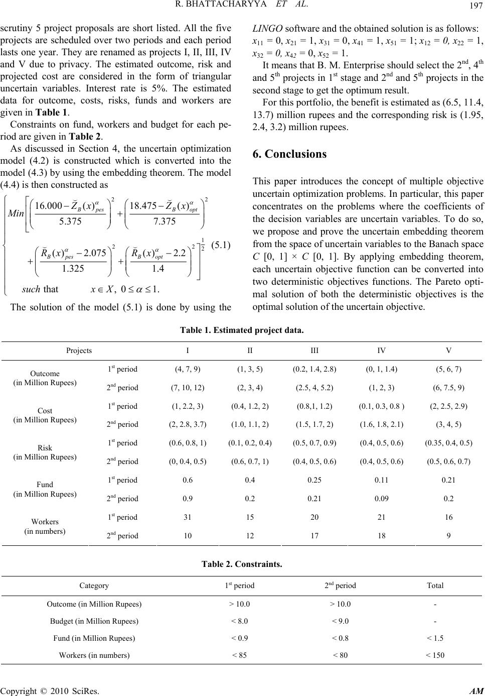

R. BHATTACHARYYA ET AL.
197
scrutiny 5 project proposals are short listed. All the five
projects are scheduled over two periods and each period
lasts one year. They are renamed as projects I, II, III, IV
and V due to privacy. The estimated outcome, risk and
projected cost are considered in the form of triangular
uncertain variables. Interest rate is 5%. The estimated
data for outcome, costs, risks, funds and workers are
given in Table 1.
Constraints on fund, workers and budget for each pe-
riod are given in Table 2.
As discussed in Section 4, the uncertain optimization
model (4.2) is constructed which is converted into the
model (4.3) by using the embedding theorem. The model
(4.4) is then constructed as
22
1
22
2
16.000( )18.475()
5.375 7.375
( )2.075( )2.2
1.325 1.4
that , 01.
BpesB opt
BpesB opt
Zx Zx
Min
Rx Rx
suchx X



























(5.1)
The solution of the model (5.1) is done by using the
LINGO software and the obtained solution is as follows:
x11 = 0, x21 = 1, x31 = 0, x41 = 1, x51 = 1; x12 = 0, x22 = 1,
x32 = 0, x42 = 0, x52 = 1.
It means that B. M. Enterprise should select the 2nd, 4th
and 5th projects in 1st stage and 2nd and 5th projects in the
second stage to get the optimum result.
For this portfolio, the benefit is estimated as (6.5, 11.4,
13.7) million rupees and the corresponding risk is (1.95,
2.4, 3.2) million rupees.
6. Conclusions
This paper introduces the concept of multiple objective
uncertain optimization problems. In particular, this paper
concentrates on the problems where the coefficients of
the decision variables are uncertain variables. To do so,
we propose and prove the uncertain embedding theorem
from the space of uncertain variables to the Banach space
C [0, 1] × C [0, 1]. By applying embedding theorem,
each uncertain objective function can be converted into
two deterministic objectives functions. The Pareto opti-
mal solution of both the deterministic objectives is the
optimal solution of the uncertain objective.
Table 1. Estimated project data.
Projects I II III IV V
1st period (4, 7, 9) (1, 3, 5) (0.2, 1.4, 2.8) (0, 1, 1.4) (5, 6, 7)
Outcome
(in Million Rupees) 2nd period (7, 10, 12) (2, 3, 4) (2.5, 4, 5.2) (1, 2, 3) (6, 7.5, 9)
1st period (1, 2.2, 3) (0.4, 1.2, 2) (0.8,1, 1.2) (0.1, 0.3, 0.8 ) (2, 2.5, 2.9)
Cost
(in Million Rupees) 2nd period (2, 2.8, 3.7) (1.0, 1.1, 2) (1.5, 1.7, 2) (1.6, 1.8, 2.1) (3, 4, 5)
1st period (0.6, 0.8, 1) (0.1, 0.2, 0.4) (0.5, 0.7, 0.9) (0.4, 0.5, 0.6) (0.35, 0.4, 0.5)
Risk
(in Million Rupees) 2nd period (0, 0.4, 0.5) (0.6, 0.7, 1) (0.4, 0.5, 0.6) (0.4, 0.5, 0.6) (0.5, 0.6, 0.7)
1st period 0.6 0.4 0.25 0.11 0.21
Fund
(in Million Rupees) 2nd period 0.9 0.2 0.21 0.09 0.2
1st period 31 15 20 21 16
Workers
(in numbers) 2nd period 10 12 17 18 9
Table 2. Constraints.
Category 1st period 2nd period Total
Outcome (in Million Rupees) > 10.0 > 10.0 -
Budget (in Million Rupees) < 8.0 < 9.0 -
Fund (in Million Rupees) < 0.9 < 0.8 < 1.5
Workers (in numbers) < 85 < 80 < 150

R. BHATTACHARYYA ET AL.
198
This paper also introduces a new model of R & D pro-
ject portfolio selection by identifying project information
like estimated future outcome, risk or estimated cost of
the projects as uncertain variables. An uncertain bi-ob-
jective optimization model, that maximizes the benefit
and minimizes the risk, is constructed. Constraints on
budget, resources and outcomes are also included in the
model to make it more realistic. The uncertain optimiza-
tion method by embedding theorem is used to solve it. A
real case study is provided for illustration.
In future, we will use the uncertain optimization ap-
proach to other real optimization problems like portfolio
selection problem, supply chain management problem,
poverty management problem etc.
For large data sets, meta-heuristic algorithms such as
tabu search, simulated annealing, ant-colony optimiza-
tion, and particle swarm optimization may be employed
to solve the non-linear programming problem (4.4).
7. References
[1] M. L. Puri and D. A. Ralescu, “Differentials for Fuzzy
Functions,” Journal of Mathematical Analysis and its
Application, Vol. 91, No. 2, 1983, pp. 552-558.
[2] O. Kaleva, “The Cauchy Problem for Fuzzy Differential
Equations,” Fuzzy Sets and Systems, Vol. 35, No. 3, 1990,
pp. 389-396.
[3] C. X. Wu and M. Ma, “Embedding Problem of Fuzzy
Number Space: Part I,” Fuzzy Sets and Systems, Vol. 44,
No. 1, 1991, pp. 33-38.
[4] C. X. Wu, “An (α, β)-Optimal Solution Concept in Fuzzy
Optimization Problems,” Optimization, Vol. 53, No. 2,
2004, pp. 203-221.
[5] C. X. Wu, “Evaluate Fuzzy Optimization Problems Based
on Bi Objective Programming Problems,” Computer and
Mathematics with Applications, Vol. 47, No. 5, 2004, pp.
893-902.
[6] M. Rabbani, M. A. Bajestani and G. B. Khoshkhou, “A
Multi-Objective Particle Swarm Optimization for Project
Selection Problem,” Expert Systems with Applications,
Vol. 37, No. 1, 2010, pp. 315-321.
[7] M. Rabbani, R. T. Moghaddam, F. Jolai and H. R.
Ghorbani, “A Comprehensive Model for R and D Project
Portfolio Selection with Zero - One Linear Goal Pro-
gramming,” IJE Transactions A: Basic, Vol. 19, No. 1,
2006, pp. 55-66.
[8] Y. Fang, L. Chen and M. Fukushima, “A Mixed R & D
Projects and Securities Portfolio Selection Model,” Euro-
pean Journal of Operational Research, Vol. 185, No. 2,
2008, pp. 700-715.
[9] S. Riddell and W. A. Wallace, “The Use of Fuzzy Logic
and Expert Judgment in the R & D Project Portfolio Se-
lection Process,” Proceedings: PICMET, Portland, 2007,
pp. 1228- 1238.
[10] H. Eilat, B. Golany and A. Shtub, “Constructing and
Evaluating Balanced Portfolios of R & D Projects with
Interactions: A DEA Based Methodology,” European
Journal of Operational Research, Vol. 172, No. 3, 2006,
pp. 1018-1039.
[11] C. Stummer and K. Heidenberger, “Interactive R&D
Portfolio Selection Considers Multiple Objectives, Pro-
ject Interdependencies, and Time: A Three Phase Ap-
proach,” Proceedings: PICMET, Portland, 2001, pp. 423-
428.
[12] J. D. Linton, S. T. Walsh, B. A. Kirchhoff, J. Morabito
and M. Merges, “Selection of R & D Projects in a Portfo-
lio,” Proceedings of IEEE Engineering Management So-
ciety, Washington, 2000, pp. 506-511.
[13] J. L. Ringuest, S. B. Graves and R. H. Case, “Conditional
Stochastic Dominance in R & D Portfolio Selection,”
IEEE Transactions on Engineering Management, Vol. 47,
No. 4, 2000, pp. 478-484.
[14] R. L. Schmidt, “A model for R & D Project Selection
with Combined Benefit, Outcome, and Resource Interac-
tions,” IEEE Transactions on Engineering Management,
Vol. 40, No. 4, 1993, pp. 403-410.
[15] O. Pereira and D. Junior, “The R & D Project Selection
Problem with Fuzzy Coefficients,” Fuzzy Sets and Sys-
tems, Vol. 26, No. 3, 1988, pp. 299-316.
[16] M. A. Coffin and B. W. Taylor, “Multiple Criteria R & D
Selection and Scheduling Using Fuzzy Logic,” Com-
puters Operations Researches, Vol. 23, No. 3, 1996, pp.
207-220.
[17] L. L. Machacha and P. Bhattacharya, “A Fuzzy-Logic-
Based Approach to Project Selection,” IEEE Transac-
tions on Engineering Management, Vol. 47, No. 1, 2000,
pp. 65-73.
[18] D. Kuchta, “A Fuzzy Mode for R & D Project Selection
with Benefit: Outcome and Resource,” The Engineering
Economist, Vol. 46, No. 3, 2001, pp. 164-180.
[19] S. Mohamed and A. K. McCowan, “Modelling Project
Investment Decisions under Uncertainty Using Possibility
Theory,” International Journal of Project Management,
Vol. 19, No. 4, 2001, pp. 231-241.
[20] Y. G. Hsu, G. H. Tzeng and J. Z. Shyu, “Fuzzy Multiple
Criteria Selection of Government-Sponsored Frontier
Technology R & D Projects,” R & D Management, Vol.
33, No. 5, 2003, pp. 539-551.
[21] J. Wang and W. L. Hwang, “A Fuzzy Set Approach for
R&D Portfolio Selection Using a Real Options Valuation
Model,” Omega, Vol. 35, No. 3, 2007, pp. 247-257.
[22] S. S. Kim, Y. Choi, N. M. Thang, E. R. Ramos and W. J.
Hwang, “Development of a Project Selection Method on
Information System Using ANP and Fuzzy Logic,”
World Academy of Science, Engineering and Technology,
Vol. 53, No. 6, 2009, pp. 411-415.
[23] E. E. Karsak, “A Generalized Fuzzy Optimization Frame-
work for R&D Project Selection Using Real Options
Valuation,” Proceedings of ICCCSA, Berlin, Heidelberg,
New York, 2006, pp. 918-927.
[24] B. Liu, “Uncertainty Theory,” 2nd Edition, Springer-

R. BHATTACHARYYA ET AL.
199
Verlag, Berlin, 2007.
[25] B. Liu, “Fuzzy Process, Hybrid Process and Uncertain
Process,” Journal of Uncertain Systems, Vol. 2, No. 1,
2008, pp. 3-16.
[26] B. Liu, “Some Research Problems in Uncertainty The-
ory,” Journal of Uncertain Systems, Vol. 3, No. 1, 2009,
pp. 3-10.
[27] X. Li and B. Liu, “Hybrid Logic and Uncertain Logic,”
Journal of Uncertain Systems, Vol. 3, No. 2, 2009, pp.
83-94.
[28] B. Liu, “Uncertainty Theory,” 3rd Edition. http://orsc.edu.
cn/liu/ut.pdf
[29] X. Gao, “Some Properties of Continuous Uncertain Mea-
sure,” International Journal of Uncertainty, Fuzziness
and Knowledge-Based Systems, Vol. 18, No. 4, 2007, pp.
383-390.
[30] C. You, “Some Convergence Theorems of Uncertain
Sequences,” Mathematical and Computer Modelling, Vol.
49, No. 3-4, 2009, pp. 482-487.