Applied Mathematics, 2010, 1, 179-188
doi:10.4236/am.2010.13022 Published Online September 2010 (http://www.SciRP.org/journal/am)
A Retrospective Filter Trust Region Algorithm for
Unconstrained Optimization*
Yue Lu, Zhongwen Chen
School of Mathematics Science, Suzhou University, Suzhou, China
Received June 8, 2010; revised July 18, 2010; accepted July 21, 2010
Abstract
In this paper, we propose a retrospective filter trust region algorithm for unconstrained optimization, which is
based on the framework of the retrospective trust region method and associated with the technique of the
multi-dimensional filter. The new algorithm gives a good estimation of trust region radius, relaxes the condi-
tion of accepting a trial step for the usual trust region methods. Under reasonable assumptions, we analyze
the global convergence of the new method and report the preliminary results of numerical tests. We compare
the results with those of the basic trust region algorithm, the filter trust region algorithm and the retrospective
trust region algorithm, which shows the effectiveness of the new algorithm.
Keywords: Unconstrained Optimization, Retrospective, Trust Region Method, Multi-Dimensional Filter
Technique
1. Introduction
Consider the following unconstrained optimization pro-
blem

min
f
x (1)
where , :
nn
x
RfR R is a twice continuously diff-
erentiable function.
The trust region method for unconstrained optimiza-
tion is first presented by Powell [1], which, in some
sense, is equivalent to the Levenberg-Marquardt method
which is used to solve the least square problems and
which was given by Levenberg [2] and Marquardt [3].
The basic idea of trust region methods works as follows.
In the neighborhood of the current iterate (which is
called the trust region), we define a model function that
approximates the objective function in the trust region
and compute a trial step within the trust region for which
we obtain a sufficient model decrease. Then we compare
the achieved reduction in f(x) to the predicted reduction
in the model for the trial step. If the ratio of achieved
versus predicted reduction is sufficiently positive, we
define our next guess to be the trial point. If this ratio is
not sufficiently positive, we decrease the trust region
radius in order to make the trust region smaller. Other-
wise, we may increase it or possibly keep it unchanged.
Since the trust region method is of the naturalness, the
strong convergence and robustness, it has been con-
cerned by many people, such as Powell [1,4,5], Schultz
et al. [6], Sorensen [7], Moŕe [8], Yuan [9] and so on. In
recent years, the trust region method has been applied to
the optimization problems with equality constraints [10],
simple bound constraints [11], convex constraints [12]
and so on. Many of convergence results have been ob-
tained, which can be seen in [13].
In Fletcher and Leyffer [14] a new technique for glob-
alizing methods for nonlinear programming (NLP) is
presented. The idea is referred to as an NLP filter, moti-
vated by the aim of avoiding the need to choose penalty
parameters, and considered the relationship between the
objective function and the constraint violation in the
view of multi-objective optimization. They make the
values of the objective function and the constraint viola-
tion to be a pair (which is called the filter), construct a
sophisticated filter mechanism by comparing the rela-
tionship between the pairs, and control the algorithm to
converge to the stationary point of the problem (1). The
results of numerical tests show that the filter methods are
very effective. Fletcher et al. [14,15], Toint et al. [16],
Ulbrich et al. [17], Wächter et al. [18,19] have combined
the idea with SQP method, trust region method, inte-
rior-point method, line search methods, respectively, and
obtained some interesting results about the filter method.
*This work was supported by Chinese NSF Grant 60873116.

Y. LU ET AL.
180
Fletcher, Leyffer and Toint [20] review the ideas above
and mention the application of the filter method in prac-
tice. In [14], they study the problem of the following
form


min
f
x,

.. 0stc x

,
where :nm
cR R is continuously differentiable func-
tion. Define the measure of the constraint violation
   
1
max 0,.
m
j
j
hcxc x


We use

() ()
,
kk
fh to denote values of


f
x and
 
hcx evaluated at k
x
. Now, we give the following
definitions about the filter methods.
Definition 1.1 A pair

() ()
,
kk
fhobtained on iteration
k is said to dominate another pair

() ()
,
ll
f
h if and
only if
()()() ()
and .
kl kl
f
fhh
Definition 1.2 A filter is a list of pairs

() ()
,
ll
f
h
such that no pair dominates any other.
We use k
F
to denote the set of iteration indices

jj k such that

()()
,
j
j
fh is an entry in the cur-
rent filter.
Definition 1.3 A pair

() ()
,
ll
f
h is said to be acce-
ptable for inclusion in the filter if it is not dominated by
any pair in the filter, that is, for any pair

() ()
,
ll
fh

k
F
,

() ()
,
kk
fh satisfies
()()() ()
or
kl kl
f
fhh (2)
In order to obtain the global convergence of the algo-
rithm, we should make f, h satisfy the sufficient reduc-
tion condition, so we strengthen the acceptable rule (2)
as

( )()()( )()
or 1
kll kl
hh
f
fhh h   (3)
where (0,1)
h

. When (0,1)
h


is very small, there
is negligible difference in practice between (2) and (3).
Definition 1.4 When the pair

() ()
,
kk
fh is added to
the list of pairs in the filter, any pairs in the filter that are
dominated by the new pair are removed, that is, we re-
move the pair

() ()
,
ll
k
f
hF which satisfies
()()() ()
and .
kl kl
f
fhh
This is called the modification of the filter.
Gould et al. [21] and Miao et al. [22] applies the filter
technique to unconstrained optimization, whose charac-
teristic is to relax the condition of accepting a trial step
for the usual trust region method, which improves the
effectiveness of the algorithm in some sense. The non-
monotonic algorithm also has the algorithm in some
sense. The nonmonotonic algorithm also has the charac-
teristic [23,24].
Recently, Bastin et al. [25] presents a retrospective
trust region method for unconstrained optimization.
Comparing their algorithm with the basic trust region
algorithm, the updating way of the trust region radius is
different, and the retrospective ratio

 
 
 
 
11
1
11 11
11
kkk
k
kkkk k
kkk
kk kkk
fxfx s
mxmx s
fxfx s
mxmxs



 






is mentioned, where


kk
mx s is the approximated
quadratic model of the objective function


f
x at k
x
.
k
s
is a solution of the following trust region subproblem

min ,
.. .
kk
k
mx s
st s

 (4)
k

is the trust region radius at the current iterate point.
In the basic trust region algorithm, the ratio k


 
 
kkk
k
kkkk k
f
xfxs
mxmx s



plays the following two roles.
1) Determine the trial step to be accepted by the algo-
rithm or not.
2) Adjust the trust region radius correspondingly.
In the retrospective trust region method, the two roles
are played by the ratio

and

, respectively. In the
basic trust region algorithm, the determination of trust
region radius is an important and difficult problem. Sart-
enaer [26] and Zhang et al. [27] present the self-adaptive
trust region methods and give some discussions about the
determination of trust region radius. Bastin et al. [25]
presents a retrospective trust region method for uncon-
strained optimization. The retrospective ratio in this
method uses the information at the current iterate and the
last iterate point, which can give the more effective esti-
mation of trust region radius. Hence, the number of
solving trust region subproblem may be decreased,
which improves the effectiveness of the method.
In this paper we present a new algorithm for uncon-
strained optimization, which is based on the framework
of the retrospective trust region method [25] and associ-
ated with the technique of the multi-dimensional filter
[21,22]. Under reasonable assumptions, we analyze the
global convergence of the new method and report the
preliminary results of numerical tests. We compare the
results with those of the basic trust region algorithm, the
filter trust region algorithm and the retrospective trust
region algorithm, which shows the effectiveness of the

Y. LU ET AL.
181
new algorithm. This paper is organized as follows. The
new algorithm is described in Section 2. Basic assump-
tions and some lemmas are given in Section 3. The
analysis of the first order and second order convergence
is given in Section 4 and Section 5, respectively. Section
6 reports the numerical results. Finally, we give some
final remarks on this approach.
2. Algorithm
In this paper, we define ()()
x
g
xfx

. At the current
iterate , (), (),
kkkk kki
x
ffxggxg denotes the ith
component of the vector k
g
. Throughout this paper,

denotes the Euclidean norm. Now, we review the basic-
trust region algorithm as follows.
2.1. Algorithm BTR (Basic Trust Region
Algorithm)
Step 0. (Initialization) Given an initial point0
n
x
Rand
an initial trust-region radius 00.

12 01

  and
12
01

 . Set :0k.
Step 1. (Model definition) Define a model function
k
m in k , where

| .
n
kkk
xR xx 
Step 2. (Step calculation) Compute a trial step k
s
for
solving trust region subproblem (4).
Step 3. (Updating iterate point) Compute ()
kk
f
xs

and the ratio
 
 
.
kkk
k
kkkk k
fxfx s
mxmx s



then,
1
1
1
, if ,
, if .
kk k
k
kk
xs
xx









Step 4. (Updating trust-region radius) Set







2
12 12
12 1
,, if ,
,, if ,,
,, if .
kk
kkkk
kk k



 

 

 

 

Set :1kk, and go to Step 1.
In the algorithm BTR, we do not give a formal stop-
ping criterion. In practice, the stopping criterion can be
installed in Step 1, such as
max
or ,
k
gepskk
where eps denotes the precision, and max
k denotes the
maximal number of iterations.
If
x
 is a local minimizer of the problem (1), then

0gx
. Motivated by the filter method, we set

g
x to be the measure of the iterate. Now we intro-
duce some definitions about the multi-dimensional filter.
Definition 2.1 We say that a point k
x
dominates an-
other point l
x
, if
for all 1,2,.
kj lj
g
gjn
Definition 2.2 A multi-dimensional filter
F
is a list
of n-tuples of the form


1,, kkn
g
g and if ,
kl
g
gF

,
then there exist two indices


12
,1,2,jj n, 12 jj

such that
11 22
and .
lj kjkjlj
g
ggg
Definition 2.3 The iterate point k
x
is acceptable for
the filter
F
if and only if for all l
g
F, there exists


1, 2,jn such that

, 0,1.
kjljg lg
g
gg n  
Definition 2.4 If the iterate point k
x
is acceptable,
then it is added to the filter and any iterates in the filter
that are dominated by the new iterate are removed, which
is called the modification of the filter.
Combining with the filter technique and the retrospec-
tive idea, we describe our algorithm as follows.
2.2. Algorithm RFTR (Retrospective Filter
Trust-Region Algorithm)
Step 0. (Initialization) An initial point 0
n
x
R and an
initial trust-region radius 00

are given.


112
123
0,1,01,01,
01.
gn

 

 


Set the initial filter
F
to be the empty set and set
:0k

.
Step 1. (Model definition) Define a model function
k
m in k

, where


| .
n
kkk
xR xx

 
Step 2. (Updating retrospective trust-region radius) If
0k

, then go to Step 3. If 1kk
x
x , then choose
1121
[, )
kkk




 . Otherwise, compute the retrospec-
tive ratio


 
1
1
.
kk
k
kk kk
fx fx
mx mx






Choose



 


1121 1
21 112
13 12
,, if ,
,, if ,,
,, if .
kk k
kkk k
kk k
 






 

 

 




Step 3. (Step calculation) Compute a trial step k
s
for
solving trust region subproblem (4) and kkk
x
xs

.

Y. LU ET AL.
182
Step 4. (Updating iterate point) Compute




.
kk
k
kk kk
fx fx
mx mx





Case 1: If 1k

 , then 1kk
x
x
.
Case 2: If 1k

  and k
x

is accepted by the filter
F
, then 1kk
x
x
 and add

kk
g
gx

 into the filter
F
.
Case 3: If 1k

  and k
x
 is not accepted by the fil-
ter
F
, then 1kk
x
x
.
Step 5. Set :1kk, go to Step 1.
Similar to the algorithm BTR, the stopping criterion
can be installed in Step 1, such as
max
or ,
k
gepskk
where eps denotes the precision, and max k denotes the
maximal number of iterations. The Hessian matrix in the
model function k m can be obtained by BFGS updating
formula or set
 
x
xk kxxk
mx sfx for all s such
that kk xs.
In the algorithm RFTR, the retrospective idea and the
filter technique are two important characteristics. The
retrospective ratio uses the information at the current
iterate and the last iterate to adjust the trust-region radius,
which can give the more effective estimation of trust
region radius. The filter technique relaxes the condition
of accepting a trial step comparing with the usual trust
region method, which improves the effectiveness of the
algorithm in some sense. From the algorithm RFTR, if
the trial point is not accepted (Case 3 in Step 5 occurs),
then the algorithm is similar to the basic trust-region al-
gorithm, whose difference is just that we use the retro-
spective idea in the algorithm RFTR. However, if the
trial point is accepted by the algorithm (Case 1 or Case 2
in Step 5 occurs), the retrospective idea and the filter
technique all play the roles.
At the iterate k
x
, if 1kkkk
x
xsx
, then the iter-
ate is called the successful iterate and the iteration index
k
x
is called successful iteration.
3. Basic Assumptions and Lemmas
In this section, we present the global convergence analy-
sis of the algorithm RFTR. We make the following as-
sumptions.
A1 The all iterates k
x
remain in a closed and bounded
convex set .
A2 :n
f
RR is a twice continuously differenti-
able function.
A3 The model function k m is first-order coherent
with the function f at the iterate k
x
, i.e. , their values and
gradients are equal at k
x
for all k,




, .
kkkxkkxk
mx fxmxfx
A4 The Hessian matrix of the model function
x
xk
m

is uniformly bounded, i.e., there exists a constant
1
umh
k such that


1,
xx kumh
mx k


holds for all n
x
R and all k.
Generally speaking, we do not need the global solution
of the trust region subproblem. We only expect to de-
crease the model at least as much as at the Cauchy point.
Therefore, we make the following assumption on the
solution k
s
of the trust region subproblem (4).
A5 There exists a constant mdc k, for all k,





22
maxmin,, min ,,
kkkk k
k
mdckkkk k
k
mxmx s
g
kg







 


 





where

 
min
1max,
| ,
min 0,().
k
kxxxk
n
kkk
kxxkk
m
xR xx
mx



 
 

By the assumptions A1 and A2, the Hessian matrix


xx
f
x is uniformly bounded on , i.e., there ex-
ists a positive constant ufh k such that, for all x

,


.
x
xufh
f
xk
Now we study the global convergence of the algorithm
RFTR. First we give a bound on the difference between
the objective function and the model function k m at the
iterate 1k
x

and k
x
. The proof of the following result is
similar to Theorem 3.1 in [25].
Lemma 3.1 [25] Suppose A1-A4 hold, then exists a
positive constant ubh k,




2
11 1 kkkubhk
fxm xk



 (5)
and if iteration 1k

is successful, that




2
11 1
kkkubh k
fxm xk




(6)
where


max ,
ubhufh umh
kkk.
As the retrospective ratio k

 uses the reduction in
k
m instead of the reduction in 1k m, we need to com-
pare their difference, which is provided by the next
Lemma.
Lemma 3.2 [25] Suppose A1-A4 hold, then for every
successful iteration 1 k

,
 


 

11 1
2
11
2
kk kk
kkkkubhk
mxmx
mx mxk
 






Y. LU ET AL.
183
We conclude from this result that the denominators in
the expression of k

 and k

are the same order as the
error between the objective function and the model func-
tion. Similar to Theorem 6.4.2 in [13], we obtain the next
result.
Lemma 3.3 Suppose A1-A5 hold, 10
k
g

and
1k
 satisfies that
2
11 1
2
1
min1, 32
mdc
kk
ubh
kg
k





 




 (7)
Then iteration 1 k is successful and
1. kk


Proof. It follows from

1
,0,1
mdc
k   and the as-
sumptions A3 and A5 that 1kubh k

. By (7),
1
1
1
.
k
k
k
g





By the assumption A5, we have that
 
1
11 111
1
11
min ,
k
kkkk mdckk
k
mdc kk
g
mxmx kg
kg


 




 




(8)
On the other hand, it follows from (5) and (7) that
 
 
1
1
11 1
11
1
1
1.
kkk
k
kk kk
ubh
k
mdc k
fxm x
mx mx
k
kg




 



 

Thus, 11k


, i.e., the iteration 1k is successful.
Next we proof the second part of the conclusion.
By

2
,0,1
mdc
k  
, we have
22
22
11
1 and 1
32 232
mdc
k







(9)
The conditions (7), (9) and the definition of 1k


in
the assumption A5 imply that
1
111
1
1 and .
2
k
mdc
kkk
ubh k
g
kg
k





Combining (8) and Lemma 3.2, we can conclude that
 
2
11111
2
111
2
2
kkkkk kkkubhk
mdckkubh k
mxmxm xm xk
kg k

 
 

(10)
By (6) and (10),




 
11 1
111
1.
2
kkkubh k
k
kkkk mdckubhk
fxm xk
mxmxkgk

 


 


(7) implies that


2121
32 1.
ubh kmdck
kkg 



i.e.,




12 11
12.
ubh kmdckubhk
kkgk 

 

Therefore,


2
11
k

  

, i.e., 2k



.
As a consequence of this property, we may now prove
that the trust region radius cannot become too small as
long as a first-order critical point is not approached. The
technique of the proof is similar to Theorem 3.4 in [25]
and Theorem 6.4.3 in [13].
Lemma 3.4 [13,25] Suppose A1-A5 hold. Suppose,
furthermore, that there exists a constant 0
lbg
k such
that klbg
g
k for all k. Then there is a constant lbd k
such that klbd k

 for all k.
4. First Order Convergence
Assume that


k
x
is an infinite sequence generated by
Algorithm RFTR. Under the assumptions (A1)-(A5), we
discuss the first order convergence of the sequence


k
x
.
At first, we define the following sets.
The set of successful iteration index


1
| .
kkk
Skx xs


The set of the iteration index which is added to the fil-
ter


| or the iterate
is added to the filter .
kkkk
A
kgxx s
F


The set of the iteration index which satisfies sufficient
descent condition


1
| .
k
Dk

 
S denotes the cardinal number of the set S. We now
establish the criticality of the limit point of the sequence
of the iterates when there are only finitely many succ-
essful iterations.
Theorem 4.1 Suppose A1-A5 hold and S

 ,
then there exists an index 0 k such that 0
k
x
x


and
x

is a first-order critical point.
Proof. Let 0 k be the last successful iteration index,
then
000 1
and , 1,2,.
kkj kj
xx j 


From Step 2 of the algorithm RFTR, we have that

Y. LU ET AL.
184
00 0
21 2
.
j
kj kjk


 
Thus,
0
lim 0.
kj
j  
It follows from Lemma 3.4 that 00
k
g.
Next, we consider the case that there are infinitely
many successful iteration. From the algorithm RFTR, we
know that
A
S. Therefore we consider the following
two cases.
1) There are infinitely many filter iterations, i.e.,
A
  .
2) There are finitely many filter iterations, i.e.,
A

 .
First, we have the following result.
Theorem 4.2 Suppose A1-A5 hold and AS,
then
lim inf0.
k
kg
 
Proof. Suppose, by contradiction, that the result is not
true, then there exists a positive constant lbg k such that
0
klbg
gk (11)
holds for all k. Denote the index set

i
A
k. It fol-
lows from the assumption A1-A5 that


k
g
is bounded.
So there exists a subsequence


1
l
i
k of


1
i
k which
satisfies
1
lim .
il
klbg
l
g
gk

 
By the definition of l
i
k, the iterate point 1
il
k
x

is ac-
cepted by the filter
F
, and for every 1
l there ex-
ists


1, 2,,
l
jn such that
11
1,1,1 .
ilili
ll l
kjk jgk
gg g 

 
 (12)
Since there is only finite choices of l j, without loss
of generality, we set l jj. In (12), we follows from
l and (11) that
1
1, 1,
00,
ii
ll
kjk jglbg
ggk 


 
which is a contradiction. Thus the result is proved.
Now, we give the result when A.
Theorem 4.3 Suppose A1-A5 hold and S

 ,
A, then
lim inf0.
k
kg  
Proof. Suppose, by contradiction, that the result is not
true, then there exists a positive constant lbg k such that
(11) holds. Since A, by the algorithm RFTR, we
have that 1k

 holds for all sufficiently large index
kS

. Denote


,1,,.
kppk S
 
It follows from the assumption A5, Lemma 3.4 and
1k

 that




11
1min,.
k
pkjj
jp
jS
lbg
kmdclbglbd
umh
fxfxfx fx
k
kk k
k




 




as long as ,pk is sufficiently large. S

 and
A

 imply that k

may be large arbitrarily, which
contradicts with the fact that


k
f
x is bounded.
By Theorem 4.1, Theorem 4.2 and Theorem 4.3, there
exists at least one limit point of the sequence


k
x
of
iterates generated by the algorithm RFTR which is a
first-order critical point.
5. Second Order Convergence
We now exploit second-order information on the objec-
tive function to discuss the second order convergence of
the sequence. We therefore introduce the following addi-
tional assumptions.
A6 The model is asymptotically second-order coherent
with the objective function near first-order critical points,
i.e.,




lim0 where lim0.
xxkxx kkk
kk
fxm xg
 


A7 There exists a constant lch k such that, for all
k,


.
xx kxx klch
mxmyk xy 
for all ,.
k
xy


Lemma 5.1 Suppose that A1-A7 hold. Suppose also
that there exists a sequence

i
k and a constant
0
mqd
k such that




20
iiii ii
kkkk kmqdk
mxmx sks

  (13)
for all i sufficiently large. Finally, suppose that lim
i
0
i
k
s

, then iteration i k is successful and
12 1
and
iii
kkk



 (14)
for all i sufficiently large.
Proof. We first deduce that every iterations i k is suc-
cessful for i sufficiently large. By the mean value theo-
rem and (13), for some k

and k

in the segment
1
,
ii
kk
xx




,

Y. LU ET AL.
185
 
 
 

 

 
 

11
1
2
1
1
2
1
2
,
iii
i
ii ii
iiiii
i
ii
iii
ii ii
kkk
k
kk kk
T
kxx kxxkkk
mqd k
xx kxx k
mqd
xxkxx kk
xx kkxx kk
fxm x
mx mx
s
fms
ks
ffx
k
fxmx
mxm







 


 
 
When i goes to infinity, by our assumption that i
k
s
tends to 0, and the bounds
and .
ii iiii
kk kkk k
x
sxs  
Combining the assumption A2 and A7, the first and
third terms of the last right-hand side tend to 0. Mean-
while, the second tends to 0 because of the assumption
A6 and Theorem 4.1, 4.2, 4.3. As a consequence, i
k

tends to 1. when i goes to infinity, and thus larger than
1

for i sufficiently large.
The residual proof is similar to Lemma 3.8 in [25].
Theorem 5.2 Suppose that A1-A7 hold and that the
complete sequence of iterates

k
x
converges to the
unique limit point
x
. Then
x
 is a second order criti-
cal point of (1).
Proof. By Theorem 4.1, 4.2, 4.3,

0gx
. We sup-
pose, by contradiction, that


*min 0 xx fx



, by
the assumption A6, there exists 0
k such that, for all


0min *
1
,2
kxxkk
kk mx

  . It follows from the
assumption A5 that
 
22
**
11
min ,
24
kkkk kmdck
mxmx sk 

 


hold for all 0
kk. Meanwhile, by the assumption we
know that 1kk k
s
xx

 tends to 0. Thus, there exists
10
kk such that, for all

1*
, min1/2,
kk
kk s   .
By Lemma 5.1, there exists 21
kk such that, for all
2
kk, we deduce that112 ,
kk
 



and 1kk .
Thus,


 


11
22
1* *
11
min,,
24
kkkkkk k
mdc k
fxfxmxmx s
k

 

 




which follows from lim k
k
x
x
  that lim 0
k
k  . This
contradicts with 1kk  for all 2 kk.Thus, *0


and therefore
x
 is a second-order critical point of (1).
6. Numerical Experiments
In this section, a preliminary numerical test of the algo-
rithm BTR, the algorithm FTR [22], the algorithm RTR
[25] and the algorithm FTR are given. The Matlab codes
(Version 7.4.0.287 R2007a) were written corresponding
to those algorithms. For the numerical tests, we use the
following trust-region radius updated form which is
proposed in Conn et al. [13].


111
1112
312
, if ,
, if ,,
max,, if .
kk
kk k
kk k
s
s


















and the following parameter settings [21,28].
1311 22
0.25, 3.5, 0.0001, 0.99,



 

 
01, min0.001,12. gn
  
The Hessian matrix of the model function is




x
xkxx k
mx fx. The termination criterion is as
following,


6
max max
10 or , 1000,
k
gnkkk


where max
k denotes the maximal iteration number.
We choose 24 test problems from [29], where “S201”
means problem 201 in Schittkowski (1987) collection
[29], 12 test problems from CUTE [25,30] and the fa-
mous Extended Rosenbrock test problem. In the follow-
ing tables, “n” means the test problem’s dimension,
“nBTR, nFTR, nRTR, nRFTR” mean the number of it-
erations of the algorithm BTR, the algorithm FTR, the
algorithm RTR and the algorithm RFTR, respectively.
“ng1, ng2, ng3, ng4” mean the number of gradient
evaluations of the algorithm BTR, the algorithm FTR,
the algorithm RTR and the algorithm RFTR, respec-
tively.
“r” means the rank of the number of iterations of the
algorithm RFTR among the four algorithms, whose val-
ues is in {1, 2, 3, 4}, where “1” means that the number of
iterations of the algorithm RFTR is the smallest among
the four algorithms, so the algorithm RFTR is the best
one among the four algorithms. “4” means that the num-
ber of iterations of the algorithm RFTR is the largest
among the four algorithms, so the algorithm RFTR is the
worst one among the four algorithms. “F” means that the
algorithm does not stop when the maximal iteration
number is achieved.
In Table 1, there are 20 test problems whose iteration
number is the smallest, 2 test problems whose rank is
second, 2 test problems whose iteration number is the
largest among 24 test problems. The numerical results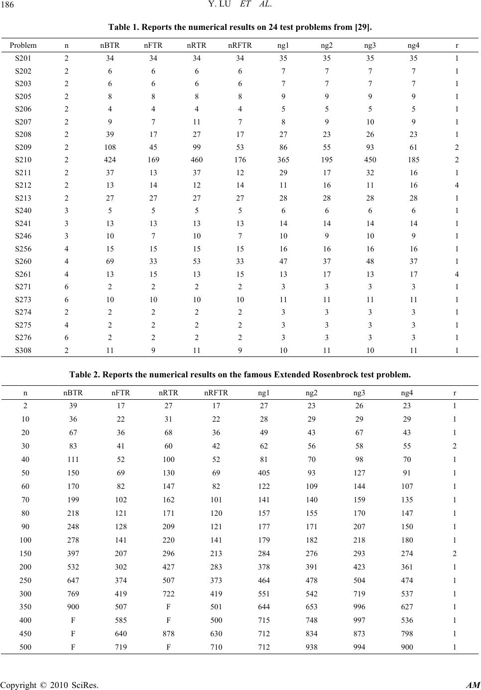

Y. LU ET AL.
186
Table 1. Reports the numerical results on 24 test problems from [29].
Problem n nBTR nFTR nRTR nRFTR 1ng 2ng 3ng 4ng r
S201 2 34 34 34 34 35 35 35 35 1
S202 2 6 6 6 6 7 7 7 7 1
S203 2 6 6 6 6 7 7 7 7 1
S205 2 8 8 8 8 9 9 9 9 1
S206 2 4 4 4 4 5 5 5 5 1
S207 2 9 7 11 7 8 9 10 9 1
S208 2 39 17 27 17 27 23 26 23 1
S209 2 108 45 99 53 86 55 93 61 2
S210 2 424 169 460 176 365 195 450 185 2
S211 2 37 13 37 12 29 17 32 16 1
S212 2 13 14 12 14 11 16 11 16 4
S213 2 27 27 27 27 28 28 28 28 1
S240 3 5 5 5 5 6 6 6 6 1
S241 3 13 13 13 13 14 14 14 14 1
S246 3 10 7 10 7 10 9 10 9 1
S256 4 15 15 15 15 16 16 16 16 1
S260 4 69 33 53 33 47 37 48 37 1
S261 4 13 15 13 15 13 17 13 17 4
S271 6 2 2 2 2 3 3 3 3 1
S273 6 10 10 10 10 11 11 11 11 1
S274 2 2 2 2 2 3 3 3 3 1
S275 4 2 2 2 2 3 3 3 3 1
S276 6 2 2 2 2 3 3 3 3 1
S308 2 11 9 11 9 10 11 10 11 1
Table 2. Reports the numerical results on the famous Extended Rosenbrock test problem.
n nBTR nFTR nRTR nRFTR 1ng 2ng 3ng 4ng r
2 39 17 27 17 27 23 26 23 1
10 36 22 31 22 28 29 29 29 1
20 67 36 68 36 49 43 67 43 1
30 83 41 60 42 62 56 58 55 2
40 111 52 100 52 81 70 98 70 1
50 150 69 130 69 405 93 127 91 1
60 170 82 147 82 122 109 144 107 1
70 199 102 162 101 141 140 159 135 1
80 218 121 171 120 157 155 170 147 1
90 248 128 209 121 177 171 207 150 1
100 278 141 220 141 179 182 218 180 1
150 397 207 296 213 284 276 293 274 2
200 532 302 427 283 378 391 423 361 1
250 647 374 507 373 464 478 504 474 1
300 769 419 722 419 551 542 719 537 1
350 900 507 F 501 644 653 996 627 1
400 F 585 F 500 715 748 997 536 1
450 F 640 878 630 712 834 873 798 1
500 F 719 F 710 712 938 994 900 1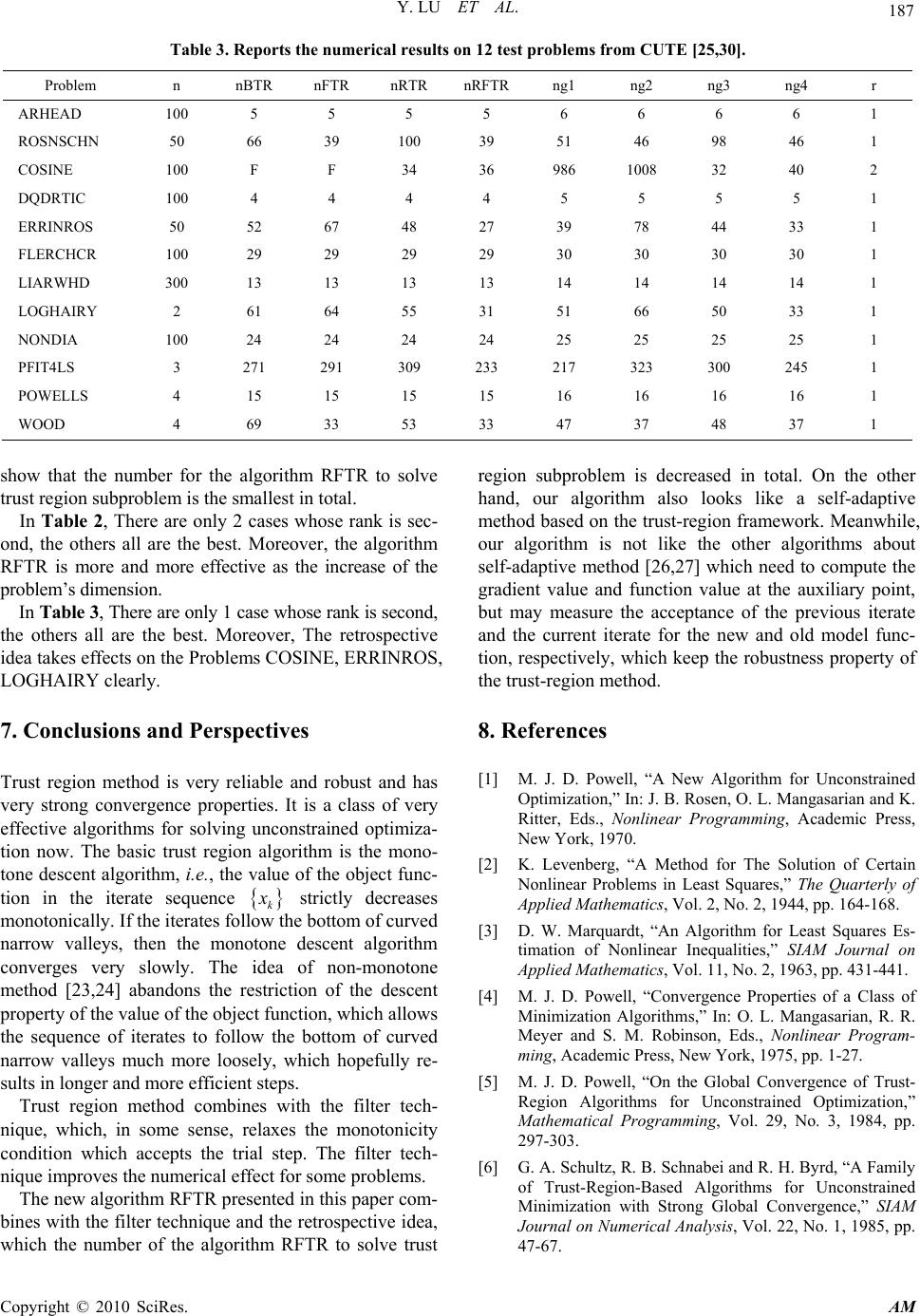

Y. LU ET AL.
187
Table 3. Reports the numerical results on 12 test problems from CUTE [25,30].
Problem n nBTR nFTR nRTR nRFTR 1ng 2ng 3ng 4ng r
ARHEAD 100 5 5 5 5 6 6 6 6 1
CHNROSNS 50 66 39 100 39 51 46 98 46 1
COSINE 100 F F 34 36 986 1008 32 40 2
DQDRTIC 100 4 4 4 4 5 5 5 5 1
ERRINROS 50 52 67 48 27 39 78 44 33 1
FLERCHCR 100 29 29 29 29 30 30 30 30 1
LIARWHD 300 13 13 13 13 14 14 14 14 1
LOGHAIRY 2 61 64 55 31 51 66 50 33 1
NONDIA 100 24 24 24 24 25 25 25 25 1
LS4PFIT 3 271 291 309 233 217 323 300 245 1
POWELLS 4 15 15 15 15 16 16 16 16 1
WOOD 4 69 33 53 33 47 37 48 37 1
show that the number for the algorithm RFTR to solve
trust region subproblem is the smallest in total.
In Table 2, There are only 2 cases whose rank is sec-
ond, the others all are the best. Moreover, the algorithm
RFTR is more and more effective as the increase of the
problem’s dimension.
In Table 3, There are only 1 case whose rank is second,
the others all are the best. Moreover, The retrospective
idea takes effects on the Problems COSINE, ERRINROS,
LOGHAIRY clearly.
7. Conclusions and Perspectives
Trust region method is very reliable and robust and has
very strong convergence properties. It is a class of very
effective algorithms for solving unconstrained optimiza-
tion now. The basic trust region algorithm is the mono-
tone descent algorithm, i.e., the value of the object func-
tion in the iterate sequence

k
x
strictly decreases
monotonically. If the iterates follow the bottom of curved
narrow valleys, then the monotone descent algorithm
converges very slowly. The idea of non-monotone
method [23,24] abandons the restriction of the descent
property of the value of the object function, which allows
the sequence of iterates to follow the bottom of curved
narrow valleys much more loosely, which hopefully re-
sults in longer and more efficient steps.
Trust region method combines with the filter tech-
nique, which, in some sense, relaxes the monotonicity
condition which accepts the trial step. The filter tech-
nique improves the numerical effect for some problems.
The new algorithm RFTR presented in this paper com-
bines with the filter technique and the retrospective idea,
which the number of the algorithm RFTR to solve trust
region subproblem is decreased in total. On the other
hand, our algorithm also looks like a self-adaptive
method based on the trust-region framework. Meanwhile,
our algorithm is not like the other algorithms about
self-adaptive method [26,27] which need to compute the
gradient value and function value at the auxiliary point,
but may measure the acceptance of the previous iterate
and the current iterate for the new and old model func-
tion, respectively, which keep the robustness property of
the trust-region method.
8. References
[1] M. J. D. Powell, “A New Algorithm for Unconstrained
Optimization,” In: J. B. Rosen, O. L. Mangasarian and K.
Ritter, Eds., Nonlinear Programming, Academic Press,
New York, 1970.
[2] K. Levenberg, “A Method for The Solution of Certain
Nonlinear Problems in Least Squares,” The Quarterly of
Applied Mathematics, Vol. 2, No. 2, 1944, pp. 164-168.
[3] D. W. Marquardt, “An Algorithm for Least Squares Es-
timation of Nonlinear Inequalities,” SIAM Journal on
Applied Mathematics, Vol. 11, No. 2, 1963, pp. 431-441.
[4] M. J. D. Powell, “Convergence Properties of a Class of
Minimization Algorithms,” In: O. L. Mangasarian, R. R.
Meyer and S. M. Robinson, Eds., Nonlinear Program-
ming, Academic Press, New York, 1975, pp. 1-27.
[5] M. J. D. Powell, “On the Global Convergence of Trust-
Region Algorithms for Unconstrained Optimization,”
Mathematical Programming, Vol. 29, No. 3, 1984, pp.
297-303.
[6] G. A. Schultz, R. B. Schnabei and R. H. Byrd, “A Family
of Trust-Region-Based Algorithms for Unconstrained
Minimization with Strong Global Convergence,” SIAM
Journal on Numerical Analysis, Vol. 22, No. 1, 1985, pp.
47-67.

Y. LU ET AL.
188
[7] D. C. Sorensen, “Newton’s Method with a Model Trust
Region Modifications,” SIAM Journal on Numerical
Analysis, Vol. 19, No. 2, 1982, pp. 409-426.
[8] J. J. Moŕe, “Recent Developments in Algorithms and
Software for Trust Region Methods,” In A. R. Bachem,
M. Grotshel and B. Korte, Eds., Mathematical Program-
ming: The State of the Art, Springer-Verlag, Berlin, 1983,
pp. 258-287.
[9] Y. X. Yuan, “On the Convergence of Trust Region Algo-
rithm,” Mathematica Numerica Sinica, Vol. 16, No. 3,
1996, pp. 333-346.
[10] M. Lalee, J. Nocedal and T. Plantenga, “On the Implenta-
tion of an Algorithm for Large-Scale Equality Con-
strained Optimization,” SIAM Journal on Optimization,
Vol. 8, No. 3, 1998, pp. 682-706.
[11] A. Friedlander, J. M. Martinez and S. A. Santos, “A New
Trust Region Algorithm for Bound Constrained Minimi-
zation,” Applied Mathematics and Optimization, Vol. 30,
No. 3, 1994, pp. 235-266.
[12] A. R. Conn, N. I. M. Gould and P. L. Toint, “Conver-
gence Properties of Minimization Algorithms for Convex
Constraints Using a Structured Trust Region,” SIAM
Journal on Optimization, Vol. 6, No. 4, 1996, pp. 1059-
1086.
[13] A. R. Conn, N. I. M. Gould and P. L. Toint, “Trust Re-
gion Methods,” MPS-SIAM Series on Optimization,
SIAM, Philadelphia, 2000.
[14] R. Fletcher and S. Leyffer, “Nonlinear Programming
without a Penalty Function,” Mathematical Programming,
Vol. 91, No. 2, 2002, pp. 239-269.
[15] R. Fletcher, N. I. M. Gould, S. Leyffer, P. L. Toint and A.
Wächter, “Global Convergence of a Trust-Region SQP-
Filter Algorithm for General Nonlinear Programming,”
SIAM Journal on Optimization, Vol. 13, No. 3, 2002, pp.
635-659.
[16] R. Fletcher, S. Leyffer and P. L. Toint, “On the Global
Convergence of a Filter-SQP Algorithm,” SIAM Journal
on Optimization, Vol. 13, No. 1, 2002, pp. 44-59.
[17] M. Ulbrich, S. Ulbrich and L. N. Vicente, “A Globally
Convergent Primal Dual Interior-Point Filter Method for
Nonconvex Nonlinear Programming,” Mathematical Pro-
gramming, Vol. 100, No. 2, 2003, pp. 379-410.
[18] A. Wächter and L. T. Biegler, “Line Search Filter Meth-
ods for Nonlinear Programming: Motivation and Global
Convergence,” SIAM Journal on Optimization, Vol. 16,
No. 1, 2005, pp. 1-31.
[19] A. Wächter and L. T. Biegler, “Line Search Filter Meth-
ods for Nonlinear Programming: Local Convergence,”
SIAM Journal on Optimization, Vol. 16, No. 1, 2005, pp.
32-48.
[20] R. Fletcher, S. Leyffer and P. L. Toint, “A Brief History
of Filter Methods,” SIAG/OPT Views and News, Vol. 18,
No. 1, 2006, pp. 2-12.
[21] N. I. M. Gould, C. Sainvitu and P. L. Toint, “A Filter-
Trust-Region Method for Unconstrained Optimization,”
SIAM Journal on Optimization, Vol. 16, No. 2, 2005, pp.
341-357.
[22] W. H. Miao and W. Y. Sun, “A Filter Trust-Region
Method for Unconstrained Optimization,” Numerical
Mathematics − A Journal of Chinese Universities.
Gaodeng Xuexiao Jisuan Shuxue Xuebao, Vol. 29, No. 1,
2007, pp. 88-96.
[23] L. Grippo, F. Lampariello and S. Lucidi, “A Non-
monotone Line Search Technique for Newton’s Meth-
ods,” SIAM Journal on Numerical Analysis, Vol. 23, No.
4, 1986, pp. 707-716.
[24] P. L. Toint, “Non-Monotone Trust-Region Algorithms for
Nonlinear Optimization Subject to Convex Constraints,”
Mathematical Programming, Vol. 77, No. 1, 1997, pp.
69-94.
[25] F. Bastin, V. Malmedy, M. Mouffe, P. L. Toint and D.
Tomanos, “A Retrospective Trust-Region Method for
Unconstrained Optimization,” Mathematical Program-
ming, Vol. 123, No. 2, 2010, pp. 395-418.
[26] A. Sartenaer, “Automatic Determination of an Initial
Trust Region in Nonlinear Programming,” SIAM Journal
on Scientific Computing, Vol. 18, No. 6, 1997, pp. 1788-
1803.
[27] X. S. Zhang, Z. W. Chen and J. L. Zhang, “A Self-Adap-
tive Trust Region Method Unconstrained Optimization,”
Operations Research Transactions, Vol. 5, No. 1, 2001,
pp. 53-62.
[28] N. I. M. Gould, D. Orban, A. Sartenaer and P. L. Toint,
“Sensitivity of the Trust-Region Algorithms to Their Pa-
rameters,” 4OR: A Quarterly Journal of Operations Re-
search, Vol. 3, No. 3, 2005, pp. 227-241.
[29] K. Schittkowski, “More Test Examples for Nonlinear
Programming Codes,” Lecture Notes in Economics and
Mathematical Systems, Springer Verlag, Berlin, Heide-
berg, Vol. 282, 1987.
[30] H. Y. Benson, “Nonlinear Optimization Models by AMPL:
Cute Set.” http://www.princeton.edu/~rvdb/ampl/nlmodels