Applied Mathematics, 2010, 1, 159-178
doi:10.4236/am.2010.13021 Published Online September 2010 (http://www.SciRP.org/journal/am)
Solidification and Structuresation of Instability Zones
Evgeniy Alexseevich Lukashov1, Evgeniy Vladimirovich Radkevich2
1Soyuz Aircraft-Engine Scientific and Technical Complex (AMNTK SOUYUZ), Moscow, Russia
2Moscow State University, Moscow, Russia
Received May 1, 2010; revised July 15, 2010; accepted July 17, 2010
Abstract
Two mathematical crystallization models describing structure formations in instability zones are proposed
and justified. The first model, based on a phase field system, describes crystallization processes in binary
alloys. The second model, based on a modified Biot model of a porous medium and the convective Cahn–
Hilliard model, governs oriented crystallization. Physical interpretation and numerical analysis are discussed.
Keywords: Solidification, Structuresation of Instability Zones, Phase Field Model
1. Introduction
Unlike the main properties of oriented crystallization,
properties responsible for the alloy structure have not yet
been studied well. At the same time, owing to recent
experimental results, many details of crystallization be-
come known. In this paper, we propose the so-called
“reconstruction” of oriented crystallization processes, i.e.,
a detailed theoretical description based on the known
main properties.
To reconstruct a process of binary alloy crystallization,
one should begin with the question why the process “can
live” in the stochastic instability. Perhaps, like in the case
of complicated systems [1], the crystallization process
can exist for a long time only due to solid structure for-
mations in instability zones. Moreover, taking into ac-
count such structure formations, we are able to explain
the solid phase growth – the crystallization mechanism.
It is known [2] that the structure formation in an alloy
obtained by the oriented crystallization method is char-
acterized by the following properties.
1) The process proceeds in a solid–liquid domain – a
dynamic porous medium–where the solid phase is repre-
sented by growing dendrites, whereas the liquid phase
occupies the space between these dendrites. According to
experimental results, the solid phase growth is of order

Ot, where t is time.
2) In the case of overlapping dendrites (in particular,
their secondary branches), the melt solidification can
lead to the contraction of melt and formation of internal
stresses and micropores.
3) In turn, a solid-liquid crystallization zone appears
because of the instability of the crystallization front
which can be caused by the following reasons:
 concentration overcooling,
 segregation of the melt components in view of the
spinodal decomposition (i.e., phase transition with
instable states) when the melt deeply penetrates
into the metastable (or even labile) domain under
high-speed (high-gradient) cooling in the inter-
phase zone.
4) Properties of a new alloy are encoded in a seed
crystal (a small piece of the solid phase) which, like the
genetic code, determines the required properties of the
crystallized part.
The experimental results concerning the distribution of
crystallization centers over the blank surface are repre-
sented in Figure 1, where it is seen that crystallization
centers are concentrated on convex parts of the surface,
but not on its concave parts. In both cases, one of the
phases grows in time, whereas the other decreases. We
also note that the picture demonstrates the structure or-
dering.
The goal of this paper is to construct mathematical
models reflecting Properties 1–4 and simulating the
structure formation in alloys and, first of all, in instability
zones. We propose two models (cf. Sections 3 and 4)
with banding structure in the zone of instability.
But, first, we emphasize that, within the frameworks
of models where structure formations in the instability
zone are not taken into account, it is impossible to obtain
the experimental order


Ot of the solid phase growth
(cf. Property 1). We illustrate this fact by considering the
well-known statistical Kolmogorov model [3] describing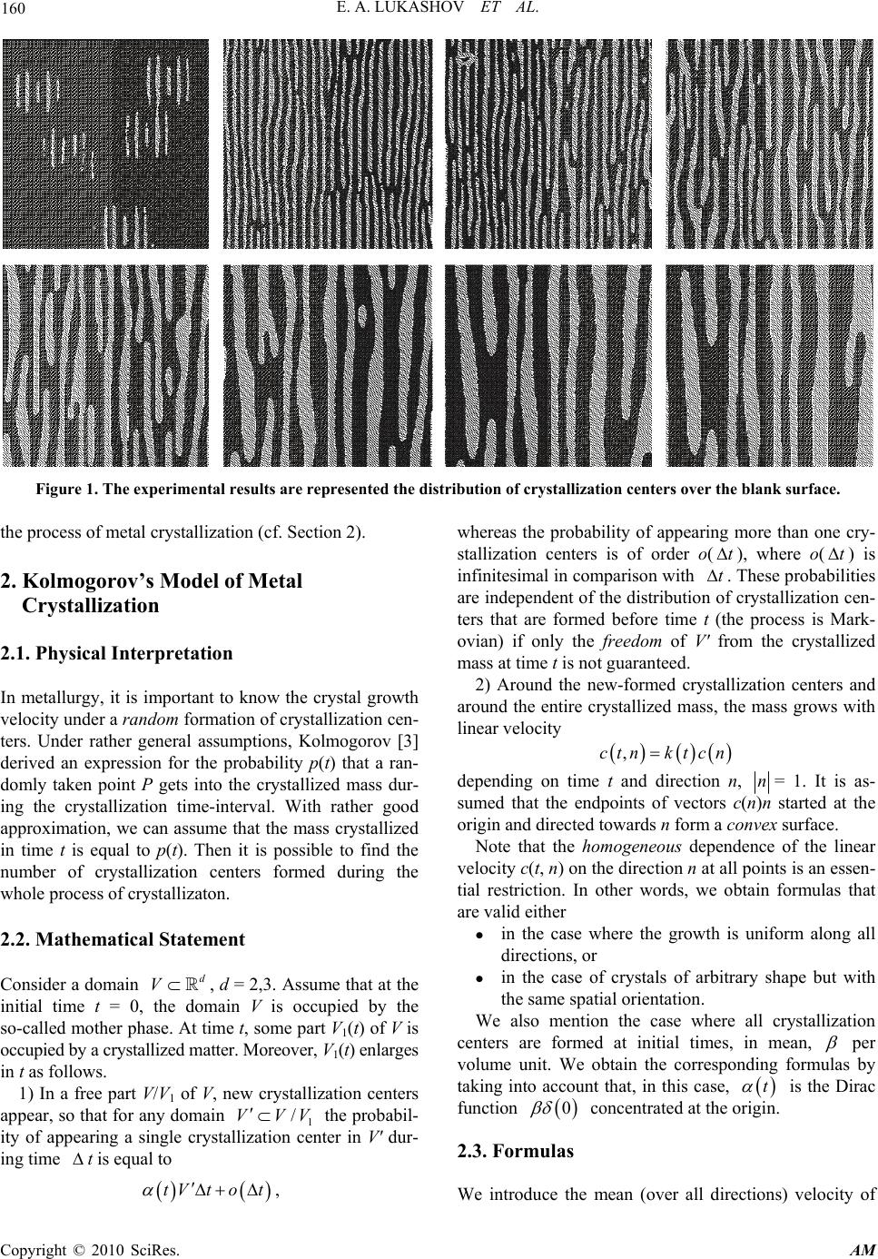

E. A. LUKASHOV ET AL.
160
Figure 1. The experimental results are represented the distribution of crystallization centers over the blank surface.
the process of metal crystallization (cf. Section 2).
2. Kolmogorov’s Model of Metal
Crystallization
2.1. Physical Interpretation
In metallurgy, it is important to know the crystal growth
velocity under a random formation of crystallization cen-
ters. Under rather general assumptions, Kolmogorov [3]
derived an expression for the probability p(t) that a ran-
domly taken point P gets into the crystallized mass dur-
ing the crystallization time-interval. With rather good
approximation, we can assume that the mass crystallized
in time t is equal to p(t). Then it is possible to find the
number of crystallization centers formed during the
whole process of crystallizaton.
2.2. Mathematical Statement
Consider a domain d V, d = 2,3. Assume that at the
initial time t = 0, the domain V is occupied by the
so-called mother phase. At time t, some part V1(t) of V is
occupied by a crystallized matter. Moreover, V1(t) enlarges
in t as follows.
1) In a free part V/V1 of V, new crystallization centers
appear, so that for any domain 1 /VVV
 the probabil-
ity of appearing a single crystallization center in V' dur-
ing time t is equal to
 
tVt ot 
 ,
whereas the probability of appearing more than one cry-
stallization centers is of order o(t), where o(t

) is
infinitesimal in comparison with t. These probabilities
are independent of the distribution of crystallization cen-
ters that are formed before time t (the process is Mark-
ovian) if only the freedom of V' from the crystallized
mass at time t is not guaranteed.
2) Around the new-formed crystallization centers and
around the entire crystallized mass, the mass grows with
linear velocity


,ctnktcn
depending on time t and direction n, n= 1. It is as-
sumed that the endpoints of vectors c(n)n started at the
origin and directed towards n form a convex surface.
Note that the homogeneous dependence of the linear
velocity c(t, n) on the direction n at all points is an essen-
tial restriction. In other words, we obtain formulas that
are valid either
 in the case where the growth is uniform along all
directions, or
 in the case of crystals of arbitrary shape but with
the same spatial orientation.
We also mention the case where all crystallization
centers are formed at initial times, in mean,

per
volume unit. We obtain the corresponding formulas by
taking into account that, in this case,

t  is the Dirac
function


0  concentrated at the origin.
2.3. Formulas
We introduce the mean (over all directions) velocity of

E. A. LUKASHOV ET AL.
161
the growth of crystallized mass c by the formula
1
=(),=2,3,
||
dd
s
ccndsd
S
where the integral is taken over the surface of unit sphere
S in d
 with center at the origin, 4S

 if d = 3 and
2S

 if d = 2. Then the following assertions hold.
1) For a sufficiently large (in comparison with the size
of a crystallization center) domain V the domain V1(t)
occupied by the crystallized phase takes the form


11
d
dd
d
Ac
Vt Ve

 (1)
If

(t) and c(t, n) are time-independent, we can set

(t) =

, k(t) = 1. In this case,
1
1
d
d
t
d




, (2)
which implies

1
1
1=1
Add
dct
d
d
Vt Ve








(3)
2) If all crystallization centers are formed at initial
times, then
 
00
dd
tt t
d
t
tkddt kd

 


  


 (4)
If, in addition, k = 1, i.e., c (t, n) is independent of t,
then
d
dt

 , (5)
which implies


11
dd
dd
Ac t
Vt Ve
 
 (6)
We see that the mass growth is of power-like order

Ot

,

= 1, 2, 3, d = 1, 2, 3.
2.4. Conclusions
The Kolmogorov model is not suitable for describing
crystallization of twocomponent mixtures. Indeed, within
the frameworks of the Kolmogorov model, the fact that
the mass growth is of power order implies that the veloc-
ity is finite at t = 0, which contradicts the initial stage of
the spinodal decomposition generating an initial distribu-
tion of crystallization centers.
3. Model of Binary Alloy Crystallization
Based on the phase field system proposed in [4] and [5],
we construct a model of binary alloy crystallization with
structure formation in the zone of instability.
A crystallization model based on the phase field con-
ception was constructed in [6], where, in particular, a
sawtooth solution to the temperature distribution prob-
lem in the phase transition domain was obtained. This
result agrees with the qualitative description of autocrys-
tallization phenomena in [7,8].
The goal of this section is to obtain a sawtooth solu-
tion to the temperature distribution problem for the fol-
lowing phase field system:

,,
x
tQ
tt
  

 
 , (7)
,= 322 

 


t (8)


00
00
,, ,
tt
x
x

 

, (9)
,=|1,=| b



 (10)
where

is the temperature;

is the specific concen-
tration of the order function, equal to 1 in the liquid
phase and to 1

in the solid phase; cons
t
=

; Q = (0,
T) ×

, where n

 is a bounded domain with
C

- boundary, n ≤ 3;


0,T

; the functions
0

and 0

are sufficiently smooth for

≥ const > 0,
and the function b

is also sufficiently smooth.
The system (7)–(10) describes slow crystallization
processes [9] with an instable domain of intermediate
aggregate state, where a structure formation appears.
3.1. Wave Train Type Solutions and Singular
Limit Problem
Here, we consider a more general case where 0BV
 ,
but 0
B
VC  1 (cf. [6]). In the case of diffusion, we say
that

is a domain of intermediate aggregate state (an
IAS-domain) if 0 ),(
0
 x weakly as 0

 in
some subdomain 0
cr

 of nonzero measure.
In accordance with [6], an IAS-domain is formed by a
large number M of domains of pure (solid and liquid)
phases of small volume of order


(i.e.,


MM  
and 0


 as 0

). The macroscopic description
of an IAS-domain can be obtained by computing the
weak limit of wave train type solutions as 0

.
We formulate conditions imposed on IAS-domains.
1) The weak limit of the order functions (,, )
x
t

 as
0

 vanishes identically in the transition zone *
t
 .
2) In the domain *
,
 t
 corresponding to the regula-
rization of the IAS-domain, the solution to the phase
field system can be described in terms of the wave train
1A function 0

belongs to the class BVC if 0

is a function o
f
bounded variation (0
B
V  ) and 0

= 1.

E. A. LUKASHOV ET AL.
162
structure. In this case, the domain  is divided into a
large number of domains of “small” volume occupied by
“pure phases” and transition zones between them.
Remark 3.1 Condition (1) means, in particular, that
for almost all
t
the limit order function

belongs to
)(BV , but ()BVC


. Condition (2) is based on
the conception proposed in [6]. According to this
conception, the wave train structure is described by a
chain of modified Stefan problems in domains of “small”
volume occupied by “pure phases” and can be used for
approximating the temperature in an IAS-domain. Such a
structure is called the diffusion of the IAS-domain.
Remark 3.2 A situation where the limit order function

vanishes on a set of nonzero measure is not good
since this case corresponds to instable solutions to the
isothermal diffusion equation. It is clear that such
solutions can exist only under rather special conditions.
Therefore, we need to impose rather restrictive con-
ditions on the geometry of domains , *
t
, as well as
on the initial and boundary conditions.
Remark 3.3 From the point of view of the theory of
distributions, free boundary problems are problems about
singularity propagation. Indeed, in the rigid-front
situation, the limit order function is a Heaviside type
function (=1

on 
t and =1

 on  t) and the
limit temperature remains continuous, but with weak
discontinuity on the free boundary   ttt=.
To formulate the singular limit problem, we suppose that
0
 is a smooth surface of codimension 1,



 =
0,
dividing  into two parts 
0 so that
00 0
=  
Let 0
 and 0  be the initial data such that
)(1=
0



outside an

-neighborhood of the surface 0

and
)(
0C
 (cf. details in [6,9]). The singular limit
problem is written as
0,>,,= tx
tt







(11)
,=|,),(=| 0
0
0= bt xx




 (12)
|=0,|=2 ,
tt
V








 

 
 (13)
.=|
1 
 V
t
t

 (14)
This problem is the well-known modified Stefan prob-
lem with the Gibbs-Thomson condition (14) on the free
boundary. Here,
 
00
0
=, ,xxx 


where []|
t
f denotes the jump in f across the free
boundary t

;

is the outward (relative to 
t)
normal to t

,

V is the normal velocity of the front t

,
t
tdiv 

|)(=

 is the mean curvature of the surface
t

, and 2/3=
1 .
We assume that
0, =t
t




i.e., the front does not intersect the fixed boundary


.
Remark 3.4 The boundary conditions (13) and (14)
can be interpreted as the Hugoniot type conditions
corresponding to the problem of propagation of strong
discontinuities of the limit order function

and the
problem of propagation of weak discontinuities of the
limit temperature

. This interpretation can be justified
as follows. As is known, the necessary conditions for the
existence of a shock wave type solution to a quasilinear
hyperbolic equation generate an instable chain of Hu-
goniot type conditions. The same instability conditions
(cf. [6]) are obtained for the boundary conditions on the
free boundary if we use the classical definition (in 

)
of a weak solution to the phase field system. The
boundary conditions in the interpretation of an IAS-
domain as the limit of wave train type solutions are
referred to as Hugoniot type conditions.
Let us describe the geometric structure. Assume that,
at 0=t, the domain

contains domains of pure
(liquid or solid) phase 0,



and also the melt domain
*
0, 
 occupied by a large number of pure phase domains
of small volume i
 0,
, Mi ,1,2,= , where
M
is
even. For the sake of simplicity, we consider the case of
quasispherical symmetry. Let i
 0,
, 1,1,=

Mi , be
interfaces of domains i
 0,
 so that
1
0, 0, 0,
=,
iii



 
0
0,0,0, 0,
=, =.
M
 


 
We denote by i D
 0, the domains bounded by i  0,

and assume that
,,0,=,
1
0,0, MiDD ii 



where
.,= 1
0,0,
0
0,   M
DD

Assume that i
 0,
 are smooth surfaces of codimension
1 such that



1
10,0,2
10,2 0,3
,,
, ,,
kk
M
cdist c
ccdist c





 

  (15)
where Mk ,1,= , (0,1)


and the constants
0>, jl cc are independent of

.
Assume that i
 0,
, Mi,0,= , satisfy the following
geometric condition.
3
0, C
i

uniformly in ][0,0


,

M and

E. A. LUKASHOV ET AL.
163
= constML

  as 0

; moreover, the surfaces
obtained after the limit passage occupy the mixture
domain *
0
 bounded by 3
C-surfaces 0

 and 0


.
Remark 3.5 If Condition (A) holds, then there exists a
function )(),( 30 Cxs

such that any i
 0,
 is a level
surface of this function.
Formula (15) shows that there are no interactions (up
to )( 


) between neighboring waves such that the
distance between them is not less than )( 1




with
any constant 0>

. Thus, for sufficiently small
t
an
asymptotic solution is expressed as the superposition of
local solutions to the rigid-front problems (with one front
i
 0,
) (cf. [6,8]) (as shown in Formula (16)).
As in the case of rigid-front solution, ci,

is a smooth
extension of the auxiliary function ),,(= htx
ii


,






00
=,, ,=,0,.
nn
ii
isxt ihsh


 
We recall that the family of functions }{ i

and )(
0
j
s,
1,2=j, is defined as a solution to the chain of modified
Stefan problems with the Gibbs-Thomson condition
,
=, ,>0,
i i
it
xt
t

 
 (17)
11 1
00
,,
|=|,
ii ii
tt 


 
  (18)
1
00
,,
|=|,
iii i
tt




 (19)
1 1
11 1
00
,,
11
||=(1)2,
i
ii
ii i
tt
ii
V





 
 



 (20)
1
00
,,
||=(1)2,
i ii
ii i
tt
ii
V





 


 (21)
,=|1)(1
1
0
1
,
1
1





 i i
ti
t
i
iV


  (22)
,=|1)( 0
,
1i
i
ti
t
i
iV


    (23)
with the initial and boundary (on  ) conditions. Here,
1,0,=Mi . We set
11
,,
==,
M
tt 

 
so that the condition (18) (the condition (21)) vanishes
for 0=i (1= Mi ). Furthermore,
i
t
i
i
ti
t
i
n
i
n
idiv
t
s
sV



,,
)(
0
1
)(
0|=,||)(|=



 


 ,
0
,=tt denotes the domain bounded by 0 ,  t
 and
 
 ,
1
,=t
M
t denotes the domain bounded by M t  ,
 and


. The small corrections ),,(
)(
1htxcj are simulta-
neously corrections of order )(

 for temperature
which can be computed as solutions to the linearized
chain of modified Stefan problems with the Gibbs-
Thomson condition (cf. [6]).
For the sake of convenience, we impose the following
condition (cf. [6]).
(A’) There exist functions ),,(
(1)
 txs and ),,(
(2)
 txs
that describe respectively the surfaces i
t  ,
 with even
and odd superscripts for 0t. We denote by i
t
 ,
 the
domain bounded by the surfaces 1
,

i
t 
and ,,
i
t


Mi ,1,= , and introduce the notation
*
,,
=1
=.
M
i
tt
i




Constructing formal asymptotic solutions, we find
() ()()
01
(,, )=(,, )(,, ),
jj j
s
xtsxthc xth  


0
=,0,,= 1,2,hj

  
so that 0|>|)( j
xs uniformly with respect to * ,  t
x
for any ]=[0, 00

 hh  and



 ,0
=,,,=,=1, =2,
=2, =21, 0.
n
ii
ti
i
x
sxthihn ik
nik iM



It is obvious that
(1) (2) 0
=0 =0
|= |=(,)
tt
s
ssx

and, with accuracy )(

,
(n )(n )
ii
i0 0i
t,
=s /|s||


 
are outward normals to i
t
D
 ,.
For fixed 0>

and sufficiently small 0>t the
classical solvability of the chain of modified Stefan
problems with the Gibbs–Thomson condition is esta-
blished in the same way as in [10]. At the same time,
based only on the limit problem below, it is impossible to
formulate the initial conditions for the temperature
),(
0
 x in such a way that these conditions have sense
as 0

because the classical solvability of the
modified Stefan problem with the Gibbs-Thomson con-
dition assumes conjugate conditions on the initial surface
i
 0,
 for any

M. However, we can overcome these
.),()(
2
1
)(
2
1
=),,(
)},,(),,(
2
{)(1)(=),,(
,
1
,,1,,1,0
0=
0
0=
1
i
t
i
ticicicici
as
ii
M
i
as
i
i
M
i
as
xtx
xhtxtx








 

(16)

E. A. LUKASHOV ET AL.
164
difficulties if find a model problem for a weak limit of
temperature as 0

. Thus, we choose the initial data
),(),0,(=| 2
10=


x
as
t (24)
),(),0,(=| 00= 

x
as
t (25)
() 0
=0
|=(,),
j
t
ssx

(26)
where ),0,(
0
 x
as , ),0,(
1
 x
as , and the smooth funct-
ions ),(
0
 xs are such that conjugate conditions are
satisfied for fixed 0>

. We will be able to specify
these conditions by obtaining the limit problem.
3.2. Limit Problem
The evolution of solutions can proceed in two different
ways depending on the initial data:
(1) (2)
=0=0
| |<0,
tttt
ss (27)
(1) (2)
=0=0
| |>0,
tttt
ss (28)
where ()
j
s
, =1,2,j are the functions in Condition
(A’).
In the case (27), the boundaries move in the opposite
directions. Consequently, the wave train type structure
exists only during a small time interval since the domain
2
,
k
t

 or 21
,
k
t


 vanishes for t


. A similar situation
for the classical Stefan problem was treated in [6]. In teh
case of the phase field system, from (27) it follows that
an “overheated” or “overcooled” domain appears in *
t

.
To find conditions for the existence of wave train type
solutions in some finite time interval independent of

,
we consider the case (28), where the boundaries move in
the same direction. Assume that the following condition
holds.
(B) There exists >0T such that for any 0tT


there exist functions (,,)
i
x
th

, =0, ,1iM

, such
that the function

,,
x
t


 (defined by i



 for
,
i
t
x

 ) is continuous and is uniformly bounded for
0
[0, ]

 . Furthermore, 1()
i
iCQ

  uniformly for
0
[0, ]

 , where ,
[0, ]
=
ii
t
tT
Q




, and 3
,
i
tC 
 .
We list some consequences of Condition (B). Since
the functions i

are smooth, it is obvious that
).(=||0
1
,
0
,
h
i
t
ii
t
i


 



Therefore, taking into account the Gibbs--Thomson law
(22), (23), we find
).(=
1
1hVVi i
t
i
i
t


Since the surfaces ,
i
t

 are smooth and 1>0
ii
VV

,
we have




000
,,,,, ,1,2
jj
sxths xthsxthj 
 (29)
where the functions 0
s
,

0
j
s
 and their third order de-
rivatives are uniformly bounded for 0
[0, ]hh. As a
consequence, we find
).(= hV i
t
i


(30)
By (30) and (22), (23), we have
,=|1)( 1
1
0
1
,
1
1





 i i
ti
t
i
iV


 
,=|1)( 0
,
1i
i
ti
t
i
iV


   
which implies
).(=|
,
h
i
t
i



From Condition (B) it follows that




11
,
,,,1,,0,,
t
x
thx tT





 (31)
where 11
i




for ,
i
t
x


.
By the Gibbs-Thomson law,

1
1
00
,,
1
11
1
1| |.
ii
ii
tt
ii i
vv
tt
ii
VV
hh












 
Since 3
,
i
tC 
 uniformly with respect to h, we
find


11i
iCQ

 
.
We need the following assertion.
Lemma 3.1 1) Let i

be partition points in the interval
[0, ]L, 01 <<<
M

, and let


1
=max
ii i
h 

.
Suppose that
M
is even,
 


0,
F
CL  , and






1
1, ii
FC


 for any =1, ,iM. Then
 
=0
1const 2.
Mi
i
i
Funiformly for M 



2) Assume that ( )([0,])
F
CL

 and ()F


2
1
([,])
ii
C

 for any =1,,iM. Then
   


0
0
1
12
2.
Mi
iM
i
F
FF h
uniformlyfor even M


 


To prove the lemma, it suffices to group the terms in
1
()( )
ii
FF



in such a way that to represent them as
differences of derivatives.
Note that for passing to the limit in the wave train as
0

, we need a suitable well-defined notion of a weak
solution. We give such a definition in accordance with
[6].
Definition 3.1 A pair of functions






212
2
0, ;0, ;,LTWL TL 






2,11 4
22
0, ;WQLTWL 




E. A. LUKASHOV ET AL.
165
is called a weak solution to the problem (49) if for any
test functions (,)
x
t

, 1 (,)=((,),,(,))
n
g
xtg xtgxt
satisfying (38) the functions

and

satisfy the
equation

 


00
=,
,0)= 0
t
Q
I
dxdt
xdx

 


 


 (32)
and the integral identity (33)
where
  

2
22
11
=,=14,
2
eWW

 


and
x
g
is the matrix with entries ()= /
x
iki k
g
gx.
We set
,,0,=,= ,
][0,
Mi
i
t
Tt
i





and ].[0,=
11 T MM  



Then we substitute (34) in the integral identity (33).
We need the following assertion.
Lemma 3.2 Suppose that (,)x

 S, 2 ()( )xC 

,
||=0


, and

,>0.
t
dist const
Then for any function

1
g
CQ

 
1
0
1
,,
lim
=,,
Q
T
s
x
gxtdxdt
A
xxgxdx















where 1 =( )
s
ts

 , 1 =| | 

,

=,,
A
xd






and T  is the domain bounded by 0  and T .
By Lemma 3.2,
))(,)(,(= 20
0=
i
i
i
t
M
i
AVsgJ



   

0.=)())(,,(1)( 1
0
0=
hhAsg ii
M
i


 



Applying assertion (a) of Lemma 3.1 to the second
sum and using (31) together with Condition (B), we find
0.=)())(,)(,(= 1
20
0=
hhAVsgJi
i
i
t
M
i







(35)
We again obtain the relation (30) since the first sum in
(35) has order )( 1 h

. Taking into account (29) and
passing to the limit as 0

, we see that (35) implies
(30) in the entire domain
**
,
0
=.
lim
tt

 

Consequently,
1*
00
0
0
=,,>0.
t
ss
sdiv xt
ts






 (36)
We consider the integral identity (32). We first com-
pute the weak limit of wave train in the derivative t


in the heat equation.
Lemma 3.3 Let
),(),,(=),,( 2
1


txtx as
where 1
as

is defined by Formula (34), and
1,,0,=,),(2
1
1
Mihcdisthc ii 



where the constants 1 c and 2 c are independent of

.
Then
)())},(1)(2({=),( 1
1
1
0=
hhCV
t
j
j
j
M
j








(37)
for any functions


1
CQ   such that


1
==
,,|= |=0,|= |=0
tT tT
gCQ gg 

 (38)
Here,
 




12
1000h
Css




is a possible contribution of the terms depending on the
first corrections to the phase 0
s
relative to h.
We set


.
k
k
kvk
FVd


 

Applying assertion (b) of Lemma 3.1 to (37), we find





,,0
tx
QQQ
Jgdxdtedivgdxdtgdivgdxdt

  

, (33)
   
10
00
,,1,,, .
2
MM
i
as as
iii
ii
x
txthx  



 




 (34)

E. A. LUKASHOV ET AL.
166
).(=),( 1
10
0
0
hhCdVdV
tM
M
M















(39)
We recall that, by Condition (B), the family


,,xt


 is bounded in 1*
2
(0, ;())
t
LTW
, uniformly
with respect to

and, consequently, *-weakly con-
verges in 1*
2
(0, ;())
t
LTW
; moreover, by (31), we have
0  
 as 0

 for *
t
x in the sense of the
2*
((0, ))
t
LT-convergence. Thus,

0
,lim,,0, .
def
t
xtxt x






It is obvious that (31) does not contradict (39) if only the
sign of the leading term of corrections (depending on

0
j
s
) of velocities is independent of j and then
1=0C. On the other hand, in the domain * t
, the limit-
ing heat equation has the free term 1
C. To verify this
fact, one should prove that


12
00
s
sh

.
The proof is given below in the spherically symmetric
case. Now, we continue computations in the integral
identity (32). Integrating by parts


0
,,0,
def
t
Q
I
dxdtx dx



 

 (40)
we find (41)
where
() =|. ii
Q



By (31) the integrals over ,
i
t

 and i

,
=1, ,iM, converge to zero as 0

. We recall that,
by Definition 3.1,

0,0 0.
t
Q
II dxdtxdx

 

 

 (42)
Taking into account (30), (39), and (41), we arrive at
the required result as 0

:
0,>,\,= *tx
tt





(43)
*
=0,, 0,
t
xt 

 (44)
* 00
0
0
=,,>0,
t
ss
sdivx t
ts






 (45)
**
|=0,|=, 0,
n
tt
Vt
n


 

 (46)
0*
=0 0
0*
0=0 0
|= (),\,
|=(),,|=,
t
tb
xx
ssxx




 
 (47)
where
 


*
0
0
=,
=,,=0,
=,,=,
tt t
t
t
xsxt
x
sxt L



 


n denotes the outward normal to *
t
, =
n
V
1
00 *
|| /|
t
sst




 , and 00 () (,0)
s
xsx.
Thus, the problem (43)-(46) can be interpreted as two
classical one-phase Stefan problems joined by Equation
(45). Such an interpretation leads to the problem about
the mixture domain for processes with surface tension (cf.
[6,8]). The conditions (45), (46) and =0  on *
t

are
conditions of Hugoniot type since they should be satis-
fied for the existence of the solution under consideration.
The operator on the right-hand side of (45) degenerates
along the direction 0
s

, i.e., along 1 y if we introduce
the new coordinates 102 =,,,
n
ysy y, where 2,,
n
yy
are the coordinates on the surface 0=
s
const . Equation
(45) is ultraparbolic. As is known [11], a homogeneous
ultraparabolic equation has no real analytic solutions
with respect to t and 1 y, except for the case where the
solution is independent of the tangent variables. Further,
we need to solve the Cauchy problem (46) for the heat
Equation (43) relative to 1 y with the initial conditions
on the surface *
t

. For sufficiently small 1 y and t
this ill-posed problem has a solution only for real ana-
lytic surfaces and initial data [11]; moreover, in this case,
the values of

on the external boundary and at the
initial time are uniquely determined by the values on




 

 

01
,,
0, ,
1*
0,
01
01
0
01
0
1
00
0
1
1
,0 ,
M
tt
Mi
t t
ii
TM
M
T
M
M
Mi
i
M
ii ii
ii
Idx dxdt
tt
d ddxdt
vv t
ddxdx
vv

 
 


 
 
 
















 







 

 

 


 

 

 
 



(41)

E. A. LUKASHOV ET AL.
167
3.3. Example of a Structured Domain
Assume that n = 3, ={,<<}
x
RrR


, where =||rx,
>0R, and *
0={ (0)<<(0)}rrr

. Then Equation
(45) becomes the first order equation

* 00
2
=, =()<<(),>0.
t
ss
rrtrrtt
trr 


 (48)
It is easy to solve the problem (48) with the initial con-
dition
0
0=0
|=().
t
s
sr
Namely,


00
0,=
s
rts r
along the characteristics


2
000
,=4,00rr trtrrr


for any smooth function 0()
s
r such that 0>0
r
s.
Now, (43), (46) with
*
=2/ |
nt
Vr

is the Cauchy problem (with respect to r) in two domains




1
2
=<< ,>0,
=<<,>0.
QRrrtt
QrtrRt


To formulate the solvability conditions for this ill-
posed problem, we recall the well-known fact (cf., for
example, [11]): for the local existence of a solution to
(43), (46) it is sufficient that the curves ()rt
 be real
analytic functions with respect to t, i.e., (0)> 0r and
2
<(0)/4tr
. Consequently, for sufficiently small 0>0

and 000 =()TT

, in the domains
 

  
*
100
*
200
=0<< ,<,
=<<0,<
Qr rrttT
Qrtrr tT






there exists a real analytic solution

to the corre-
sponding Cauchy problem. Thus, in order to solve the
limit problem (43)-(46), we need to impose the following
condition.
(C) Suppose that  is a spherically symmetric layer
in 3
, the initial and boundary data of the problem
b
tt
t
tt
xx




=| 1,=|
),,(=| ),,(=|
=
,=
0
0=
0
0=
322




(49)
are spherically symmetric, and

0
0, =,||=,
i
i
x
xr


where RrrrR M<<<<<<0 00
1
0
0. Assume that
00
1= jj
rrh
 and the differences 0 0
rR

 and 0
M
Rr


are sufficiently small; moreover, 0()
s
r is real analytic,
0/>0sr , 0()
x

and b

are special data corre-
sponding to the solution to the Cauchy problem for the
heat Equations (43), (46).
We show that Condition (C) implies Condition (B)
and the equality 1=0C in (39). For this purpose, we
return to the main problem (cf. (17)-(23))
,
=, ,>0,
i
i
it
xt
t

 
 (50)
11 1
00
,,
|=|,
ii ii
tt 


 
  (51)
1
00
,,
|=|,
iii i
tt




 (52)
1
1
11 1
00
,,
11
||=(1)2,
i
ii
ii i
tt
ii
V





 
 



 (53)
1
00
,,
||=(1)2,
i
ii
ii i
tt
ii
V





 


 (54)
,=|1)( 1
1
0
1
,
1
1





 i i
ti
t
i
iV


  (55)
.=|1)( 0
,
1i
i
ti
t
i
iV


    (56)
Let =(,)
ii
th

 be functions such that ,=
i
t 

{,=(, )}
i
rrth

. In the spherically symmetric case, we
have
.2/= i
i
t
 
Therefore, taking into account (30) and choosing i

directed in the opposite direction relative to the normals
(with respect to ,
i
t
D

), we find
).(2/= hVi
i

 

We make the change of variables =/
ii
wr

. Then
the equality
,
=, , >0
i
tt
xt

 
takes the form
 

2
1
2
=,, ,>0.
ii
ii
ww
rttt
tr


 
 (57)
Since
,)/2(=),(12=1hVvhvV i
i
ti
def
ii
i
i

 
the conditions (51), (54) can be written as follows:


1
11 1
00
,,
||=141,
i
ii
ii i
tt
ww hv
rr



 


 (58)


1
1
00
,,
||=141,
i
ii
ii i
tt
ww hv
rr




 


 (59)

E. A. LUKASHOV ET AL.
168
11 1
00
,,
|=|,
ii ii
tt
ww

 
  (60)
1
00
,,
|=|.
iii i
tt
ww


 (61)
We show that the problem (57), (58) has a solution
satisfying the following properties:
1) )(= hwi uniformly with respect to i,
2) for any
t
the values

ˆ1i
i
iirp
ww

 are deter-
mined, with accuracy )(2
h

, by the values of some
function


1
0
ˆ,
iM
wC

  on the grid 0 {,,}
M

 .
We note that the first property is related to (56) and
(30).
We look for a solution i w to the problem (57), (58)
in the form


 
1
=,,,
iiiii
war btutrh 

 (62)
where the first two terms correspond to the Stefan condi-
tion (58) and i u is a solution to the following chain of
problems:
2
1
2=,=1,,,
ii
iii
uu
abi M
tr






 (63)

1
1= =
|=0, |=0,
=0,,.
jj
jjrr
jj
uu
uu rr
jM










(64)
We note that this chain is similar to that considered in
[12] and differs by only the dependence of 1 =
iii i
f
ab 




in (63) on
t
. However, because of this dependence, it is
obvious that the contribution of this chain to the solution
is of order )( 2 h

.
To solve Equation (63), we first compute the coeffici-
ents i a and i b. From (58) and (63) it follows that


1
1
=2 11,=0,
i
ii
ahvb





12
12
=2
=2111,
=2, ,.
jk
jkk
kk
k
bhvhv
jM





 



Assume that


01
,,,, 1,2,
j
sxthsxthj 
 (65)
where the functions

0
j
s
 are defined in (29). At the first
glance, this assumption can lead to a contradiction in the
equation for velocity correction (the linearized Gibbs-
Thomson equation for

0
j
s
) if the functions i

com-
puted under this assumption do not satisfy Conditions 1)
and 2) However, it turns out that there is no contradic-
tion.
Denote by (,,)Rzth a solution to the equation


01
,,=.
s
RthsRtz
By construction, =(,,)
iRihth

and, uniformly with
respect to i up to order )(h, the functions i v

are
traces of some 1 C-function v on the surfaces =i r

.
We note that />0Rz

. Furthermore,
).(=)(|1)(2= 2
2)(=
2=
hh
z
R
hb khz
k
j
k
j




By Lemma 3.1, the last estimate is uniform with re-
spect toj. Further,
),(=)()2(1)2(= 23
11
1
2hhbb jjj
j
jj  



(66)
and this estimate is also uniform with respect toj. Now,
we see (67)
Furthermore, from (66) and Lemma 3.1 it follows that
)(= 2
2hbb jlj  
uniformly with respect to j and l. In particular, from
this estimate, the equality (67), and the condition 1=0b
we find
).(=),(|2=2
12
2
1)(2=2 hbh
z
R
hblhlzl  


We consider a broken line  such that its linear
parts are defined as 1 ()
iii
arb



 on the segments
1
[,]
ii


. It is obvious that i
b are the values of  at
the points 1 =i r


. Consequently,  is not symmetric
with respect to the zero line (it is directed toward to the
domain of positive values). However, the broken line can
be centered by decreasing its values =(1)
|zhi
R
hz


 in
each segment 1 [,]
ii


. It is obvious that this is
equivalent to the existence of functions
),,(=
|= htrzz
z
R
hm

in . Here, =(,,)zzrth satisfies the equation
(,,)=Rzth r.
We set
.=,=
1muUm ii 


Then for i
U we have the problem of the form (63)
with the right-hand sides

2
11
2
=,,.
iii iii
mm
Ga br
tr




 


 (68)
).(|))(
2
(1)2(=3
1)(=
2
2
22
1
1hRv
z
h
z
Rh
z
R
hbb hjz
j
jj 








 

 (67)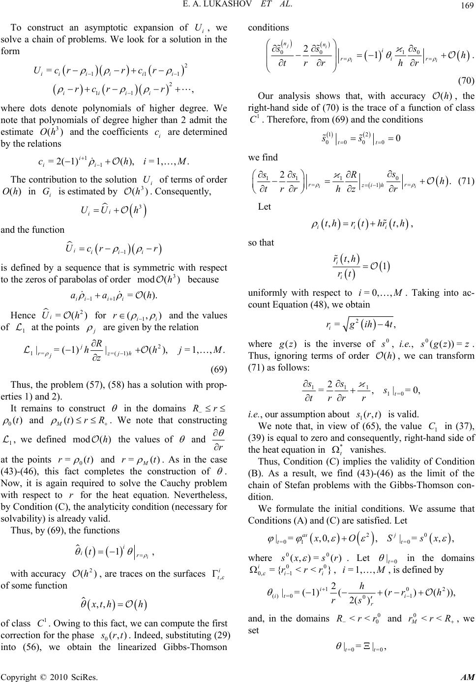

E. A. LUKASHOV ET AL.
169
To construct an asymptotic expansion of i
U, we
solve a chain of problems. We look for a solution in the
form

 
2
111
2
11
=
,
iii iii
iiii
Ucr rcr
rcr r
 




 
where dots denote polynomials of higher degree. We
note that polynomials of degree higher than 2 admit the
estimate 3 ()Oh and the coefficients i c are determined
by the relations
.,1,=),(1)2(= 1
1Mihc i i
i





The contribution to the solution i
U of terms of order
)(hO in i G is estimated by )(3
h

. Consequently,


3
i
i
UU h
and the function


1
iiii
Ucr r 


is defined by a sequence that is symmetric with respect
to the zeros of parabolas of order )(mod 3 h

because
).(=
11 haa iiii 


 
Hence

2
=()
i
Uh for ),(1ii r




and the values
of 1  at the points j

are given by the relation
.,1,=),(|1)(=| 2
1)(==1 Mjh
z
R
hhjz
j
j
r 




(69)
Thus, the problem (57), (58) has a solution with prop-
erties 1) and 2).
It remains to construct

in the domains Rr



0()t

and ()
MtrR


 . We note that constructing
1
, we defined )(modh the values of

and r



at the points )(=0tr

and )(= trM

. As in the case
(43)-(46), this fact completes the construction of

.
Now, it is again required to solve the Cauchy problem
with respect to
r
for the heat equation. Nevertheless,
by Condition (C), the analyticity condition (necessary for
solvability) is already valid.
Thus, by (69), the functions

 
1i
i
ir
t



 ,
with accuracy )( 2 h

, are traces on the surfaces i
t  ,

of some function


,,
x
th h  
of class 1
C. Owing to this fact, we can compute the first
correction for the phase 0(,)
s
rt . Indeed, substituting (29)
into (56), we obtain the linearized Gibbs-Thomson
conditions



 
00 0
1
21
ji
ii
nn
i
rir
sss h
trr hr




 

 

 

 .
(70)
Our analysis shows that, with accuracy )(h, the
right-hand side of (70) is the trace of a function of class
1
C. Therefore, from (69) and the conditions
 
12
000 0
0
tt
ss




we find


0
111
1
2.
ii
rr
zih
s ss Rh
trrhz r
 

  

 

 

 (71)
Let




,,
iii
thr thr th  
,
so that


 
,1
i
i
rth
rt 

uniformly with respect to =0,, iM. Taking into ac-
count Equation (48), we obtain

2
=4,
i
rgiht
where )(zg is the inverse of 0 s, i.e., zzgs =))((
0.
Thus, ignoring terms of order )( h, we can transform
(71) as follows:
0,=|,
2
=0=1
111
t
s
rr
s
rt
s





i.e., our assumption about 1(,)
s
rt is valid.
We note that, in view of (65), the value 1
C in (37),
(39) is equal to zero and consequently, right-hand side of
the heat equation in *
t
 vanishes.
Thus, Condition (C) implies the validity of Condition
(B). As a result, we find (43)-(46) as the limit of the
chain of Stefan problems with the Gibbs-Thomson con-
dition.
We formulate the initial conditions. We assume that
Conditions (A) and (C) are satisfied. Let






20
=0 1=0
|=,0,,|= ,,
as j
tt
xO Ssx

 
where )(=),( 00 rsxs
 . Let 0= |t

in the domains
}<<{= 00
10,ii
irrr 


, Mi ,1,= , is defined by
)),()(
)2(
(
2
1)(=| 20
1
0
1
0=)( hrr
s
h
ri
r
i
ti 

 


and, in the domains 0
0
<<rrR and  RrrM<<
0, we
set
=0 =0
|=|,
tt



E. A. LUKASHOV ET AL.
170
where  is a solution to a special Cauchy problem
(relative to
r
) for the heat Equation (43).
Theorem 3.1 Under the above assumptions, there
exists an asymptotic solution to the phase field system
satisfying Condition (B), and it is possible to pass to the
limit in (49) as 0

in the sense of Definition 3.1.
The limit problem
*
=, \,>0,
t
xt
t
 
 (72)
*
=0,, 0,
t
xt   (73)
*
00
0
0
=,,>0,
t
ss
sdivx t
ts






 (74)
**
|=0,|=, 0,
n
tt
Vt
n


 

 (75)


0*
=0 0
0*
0=0 0
|=,\ ,
|=,,|=,
t
tb
xx
ssxx




 
 (76)
where
 


*
0
0
=,
=,,=0,
=,,=,
tt t
t
t
xsxt
x
sxt L



 


n denotes the outward normal to *
t
,=
n
V
1
00 *
|| /|
t
sst


 and 00
() (,0)
s
xsx, possesses a
solution, at least for sufficiently small (but independent
of

) time.
The above case can be explained by the fact that,
outside the layer 0
M
rrr , the order function of the
original problem takes different values: 1


 for
0
<rr and 1

 for M
rr >. It is obvious that all the
arguments remain valid in the case where

takes the
same values (1

 or 1

) for ],[0M rrr
. This
means that
M
is odd. Then we again obtain a limit
problem of the form (72)-(75). The limit passage can be
justified in the same way as above, by solving a chain of
problems which can be reduced to the chain of problems
(63). In both cases (
M
is even or odd), the problems are
ill-posed. However, as was noted in [6], such a wave
train type structure appears in numerical experiments as
solutions to the phase field system with the initial data
0=
0
 for RrR

 and


0
=0
0
0
=0
11,M is odd,
=
1,M is even.
Mjj
j
Mjj
j
rr
th
rr
th





 











Figure 2(b) presents the graphs of solutions to the
phase field system with spherically symmetric initial data
for =19M and 2 =10 

at different times. One can
see that the temperature in the mixture domain is of
sawtooth form. Such a function is the leading part of the
asymptotic expansion (62) of the solution to the chain of
modified Stefan problems with the Gibbs-Thomson con-
dition. In the numerical analysis performed by O. A. Va-
sil’eva, =0

on the external boundaries. This leads to
an effect presented in the figure for time =0.02t: the
sawtooth structure begins to break down under the in-
fluence of boundary data. However, the order function is
more stable and preserves its shape.
Figure 2(a) presents the graphs of solutions to the
phase field system with spherically symmetric initial data
for =7M and 2 =10 

at different times. The tem-
perature has sawtooth shape in the IAS-domain, whereas
it is periodic with amplitude =1 l at center. Such a
function is the leading part of the asymptotic expansion
(62) of the solution to the chain of modified Stefan prob-
lems with the Gibbs−Thomson condition. The sawtooth
structure “moves” to the center and begins to break down
under the influence of nonspecial boundary data. The
order function preserves its shape in this case.
Figure 3(a) presents the graphs of solutions to the
phase field system with spherically symmetric initial data
for =7M and 2
=10 

at different times. Figure 3(b)
presents the graphs of solutions to the phase field system
with spherically symmetric initial data for =19M and
2
=10 

at different times.
3.4. Comments and Conclusions
Based on the phase field system, it is possible to detect a
banding structure formation in instability zones. How-
ever, to construct the mathematical model, we need to
impose some restricted conditions.
1) The existence conditions are very restrictive, which
can be explained by the geometry of domain

and the
initial and boundary conditions. Note that the initial and
boundary data are determined by the solution to the limit
problem.
2) A standard definition of a weak solution can turn
out to be not suitable. However, we can avoid these di-
fficulties by introducing a special definition of a weak
solution, which is important for nonlinear problems.
3) As was shown, a wave train type solution exists
only for special boundary and initial data providing the
existence of an asymptotic solution to the chain of Stefan
problems with the Gibbs-Thomson condition for suffi-
ciently small (but independent of

) times. This fact
allows us to pass to the limit of the chain of Stefan prob-
lems with the Gibbs−Thomson condition (in the sense of

E. A. LUKASHOV ET AL.
171
r
r
r
r
r
r
r
r
r
r
r
r
θ

θ

θ

θ

θ

θ

Figure 2. (a) Presents the graphs of solutions to the phase field system with spherically symmetric initial data for =7M and
2
=10 
 at different times; (b) Presents the graphs of solutions to the phase field system with spherically symmetric initial
data for =19 M and 2 =10 
 at different times.
Definition 3.1) and derive the limit problem (43)-(46).
4) As we shown in the above examples, the tempera-
ture (,, )
x
t

 is small (0

 as 0

) and has
special “periodic” structure in the stratified domain.
5) Even in the rigid-front case, the solid phase growth
is of order ln(1/ )t, which is lower than the order ob-
tained in experimental way.
Thus, a banding structure in the phase stratification
domain of a binary alloy was constructed under ex-
tremely restrictive conditions on the geometry of domain
 and the initial and boundary conditions. Furthermore,
the order ()Ot of the solid phase growth obtained in
experiments is not achieved in this model. In view of
these facts, it is necessary to look for other mathematical
models describing qualitative experimental properties of
crystallization. In the following section, for such a model
we consider the convective Cahn-Hilliard equations in a
porous medium of an overcooled melt.
4. Oriented Crystallization Model
There is a huge experimental literature on various struc-
ture formations in melt crystallization. Based on experi-
mental results, one can conjecture that complex structure
formations in crystallization are caused by the evolution
of instabilities during phase transition processes which,
in turn, is caused by different reasons and can be realized
in different ways. We list some of such reasons.
1) concentration overcooling,
2) convective flows deforming the temperature field
(gravity and thermocapillary convection),
3) phase stratification.
In addition, elastic properties of the solid phase, thin
phase boundary, and adsorption phenomena can also

E. A. LUKASHOV ET AL.
172
contribute to this effect.
4.1. Modified Convective Cahn-Hilliard Model
in a Porous Melt
To construct a mathematical model governing the recon-
struction of oriented crystallization (cf. [7,8]), a modified
Biot model of a porous medium [13] was used for de-
scribing a liquid-solid zone and the convective Cahn-
Hilliard model of spinodal decomposition [14,15] was
used for describing segregation. In the model, we con-
sider a binary eutectic alloy. For variables we take
the concentration of the component A or the compo-
nent B of the binary alloy,
the temperature,
the growth velocity of the solid phase,
the contraction,
the convection velocity of the liquid phase.
The model includes the laws of conservation of mass
and impulse for liquid and the law of conservation of
total impulse for liquid and solid phases.
In accordance with the physical interpretation, the
model also includes a modified Cahn-Hilliard equation
[14] and the heat equation [7], regarded as a generaliza-
tion of the Stefan problem [9]. Using a nonisothermic
modification of the Cahn-Hilliard model, proposed in [7],
we can construct a model that take into account the fol-
lowing physical effects.
Because of crystallization and melting, the tempera-
ture can vary. In turn, variations of temperature lead to
variations of velocity and changes of the medium com-
position.
An equilibrium phase transition is realized at the
melting temperature, whereas a nonequilibrium phase
transition can be realized at different temperatures de-
pending on the depth of penetration into metastable or
labile regions. This fact shows that the modified
Cahn-Hilliard model should include temperature-depen-
dent parameters. Then both heat-mass transfer equations
will govern mutually dependent processes.
The model reflects the structure of a liquid-to-solid
transition zone of the crystallization front. It consists of
an outer viscous layer (the hydrodynamic Prandtl layer)
and a diffuse layer (the Nernst diffusion layer). In the
case of a condensed system, the thickness of the Nernst
layer is less than the thickness of the Prandtl layer by
three orders and the heat-mass transfer laws can be as-
sumed to be linear (the Fick and Fourier laws). On the
boundary of the diffuse layer, near the solid phase, the
volume strongly varies while a liquid-to-solid transition.
Therefore, it is necessary to take into account elastic
forces, which can be done within the framework of con-
tinuum mechanics.
We introduce the following notation:
c is the mole concentration of the component B in
the binary alloy (In our case, the mole concentration of
Sn in the liquid phase),
z
is the contraction,
l
w is the convection velocity of the liquid phase,
u is the averaged displacement in the solid phase,
s
w is the mean growth velocity of the solid phase,
v is the averaged fictitious displacement in the liquid
relative to the solid phase,
T is the temperature.
Furthermore, we set
=.
ls
www
4.2. One-Dimensional Case
In this case, the model is represented (cf. [8]) by a sys-
tem of differential equations which can be divided into
the three subsystems:
 


2
=, =,
=2 ,
= ,
s
tt
sl
txx
tx
ls l
addtxx x
t
uw vw
ww MuMvg
wwDwMuMvg

 
 








(77)




=0,
ll ss
tx x
ww  

 (78)








, =)(
,]))),(()),((
)2(),(([=)(
0
2
4
1
2
2
xxt
xxxxxxxx
cxDxkrt
TDcT
cTcFcTcF
uTcFMcccwc



(79)
This system describes processes in the diffuse and
Prandtl layers in dimensionless variables c, T, l w,
s
w, u, v,
z
.
The system (77) is a model of wave propagation in a
porous skeleton filled with a liquid (a simplified version
of the Biot model).
The system (78) is the continuity equation and de-
scribes the evolution of contraction.
The system (79) presented by the convective Cahn-
Hilliard model and the heat transfer equation describes
the formation and growth of Gibbs grains.
Note that we use equations of continuum mechanics to
describe processes in the Prandtl layer, whereas for dif-
fusion and heat processes we use the modified Cahn-
Hilliard model where hydrodynamic processes and elas-
tic-plastic state of the solid phase are taken into account.
Let’s note that all constructions of the previous chapter
were maded for this one-dimensional case but more
technically.

E. A. LUKASHOV ET AL.
173
The model contains a number of dimensionless para-
meters. The elasticity modulus of the solid phase


2=  is assumed to be a function of concentration
and temperature: ),(= Tc .
The parameter
z
is expressed by the formula
=,
s
i
VV V
zV

where V is the total melt volume, s V is the current
volume of the solid phase, and l V is the current volume
of the liquid phase.
The concentration c is expressed as
=,
s
B
B
l
l
mM
cmM
where A
M (B M) is the atomic mass of the component
A
(B) and l
M
is the averaged atomic mass of the
melt: BA
lcMMcM  )(1= .
The extra variable )(cy of the form B
l
Bmmy /= is
expressed in terms of concentration as follows:
 
=,
1
qc
yc cQ (80)
which implies
 


,= ,
11
lqyc
cz R
zR yc


 
where 2/3 )))((1  cy is a bound for the surface of the
solid phase in the liquid-solid region, 1  is a parameter,
== 0,74,==0,25,==1,75
Sn PlPl
sSnSn
mmM
RqQ
Vm M

are constants, and we adopt the normalization condition
==1.
s
B

Further,

is the mean density.
6,2=M is the mobility (fluidity) of the liquid.
2
 is the inverse of the relaxation time of fluidity
(estimated as 3 10    ),
1/30= g is the acceleration of gravity,
D is the interphase friction coefficient, estimated as




2/3
/1/
1
=1 1,
TT
De eyc


 
where 1=, 5,=
1

D
M is the diffuse mobility of the component B
(estimated as TM D1/= ),
 is the ratio of the melting enthalpy to the heat
capacity of the solid phase at a constant pressure.
The function
F
determines steady, metastable, and
labile states of the system “melt-alloy” depending on the
composition and temperature. The function
F
can be
approximated by a cube polynomial in c at a fixed
temperature:






0
3
0
,
,=
,,
cr
cr
cccccTT
FcT
ccT T

 




where KT 400=
0 and cr
cc,
 are functions of temp-
erature
T
which will be specified below,
minmax minmax
,= 233,15,=456,15.TTTTKTK


We define three concentration values:
min
c equals to )( min Tc ,
mid
c equals to )(min Tccr ,
0
c equals to mid c in our experiment.
We set
min =0,04,=0,43. mid
cc
We introduce )(Tc as the roots of the equation
2
=,
clustclust clust
Tc c  
where

min 0
0
2
min 0
2
00
=,=2,
=
clustclust clust
clust clust
TT c
cc
Tc






and define )(Tccr as a linear function.
The function 1000),,(
1

TzcF is interpreted as vi-
scosity. At the first step, it is assumed to be constant. The
structure of the interphase boundary at atomic level is
characterized by the function 2 F. We set 0
2

F and
4
10=   in the numerical experiment.
The model also contains some additional relations
dictated by the physical interpretation of the problem. In
particular, the model contains the “extra” density add

such that



1/3
=,
1
l
add
z
yc
 

 (81)
where 0,055=

and, as a rule, )(z

is small for
small
z
.
4.3. Numerical Analysis of the Model
Describing Oriented Crystallization.
One-Dimensional Case
The numerical results obtained by Rykov and Zaitsev [16]
are presented in Figures 3(a-c). Note, that the spatial
x
-axis is directed upward, whereas the
t
-axis is
directed rightward along the horizontal line.
The systems presented in Figures 3(a-c) differ by the
value of the parameter . The numerical results show

E. A. LUKASHOV ET AL.
174
(a) (b) (c)
Figure 3. Numerical simulation of the model describing oriented crystallization (one-dimensional case). The spatial x-axis is
directed upward, whereas the t-axis is directed rightward along the horizontal line.
that the balance of convective and diffusive terms
generates a modulated wave of formation of crystal
grains, which differentiate the spinodal decomposition
mechanism from the classical case where the Cahn-
Hilliard model possesses a periodic solution.
4.4. Comments
1) In our model, for the sake of simplicity, we assume that
porosity is constant, passing its functions to the contrac-
tion z. On this stap of the model construction we will elu-
cidate the change range of the porosity when the modifica-
tion of Biot model don’t lose the hyperbolicity. It allow us
on the next stap to pass to porosity as a problem variable,
expressed the contraction as the function of porosity.
2) In the model (77)-(79), the convention is equal to
zero at the initial time, 0=| 0=t w, and then it can be
regarded as reaction to 1) the force of interphase friction
between liquid and solid phases and 2) the gravity force.
Thereby we specify the effective force in the convective
Cahn-Hilliard model [14,15].
3) The initial distribution of crystal grains (which,
unlike [14], is not given here) depends on only contraction,
whereas the further distribution is determined by the proc-
ess. So, no restrictive conditions are imposed on the ini-
tial-boundary data, unlike the case of the phase field system
and the one-dimensional convective Cahn-Hilliard model.
4) In the subsystem (79), we took into account the re-
sults of [17]. Note that the above constructions remain
also valid for the modified model (77)-(79) obtained
from the two-dimensional model (cf. below) in the ra-
dial-symmetric case.
4.5. Two-Dimensional Case
Introduce the notation:
c is the mole concentration of Sn in the liquid
phase,
z
is contraction,
l
w is the liquid phase velocity
l
u is the averaged displacement in the solid phase,
s
w is the mean growth velocity of the solid phase
(the averaged velocity of microfronts),
=
s
l
ww w

is the averaged fictitious displacement in
the liquid phase relative to the solid phase,
T
is the temperature.
The system of two-dimensional equations can be writ-
ten in the form




1122
=, =,
s
ss s
tt
uwu w (82)




1122
=,=,
tt
uwu w (83)
11
2
1
2
2
12
12
() ()
=[(( ,)2( ,)())()
((, )())()
()(( )())]
[(,)(( )())],
st lt
s
x
sy
xyx
sys xy
ww
cTcTM Tu
cTM Tu
MT uu
cT uu










(84)
22
12
2
1
2
2
12
() ()
=[( ,)(()() ]
((,)())( )
[((, )2(, )())()
()(()() )] ,
st lt
sys xx
sx
s
y
xyy
wwg
cT uu
cTM Tu
cTcTM Tu
MT uu












(85)
111
1212
()()= (,)
[()((()() )()())))],
ls taddlt
s
xsyxyx
wwDcTw
MT uuuu






(86)
22 2
1212
()()=(,)
[()((()() )()())))],
lstadd ltl
s
xsyxyy
wwgDcTw
MT uuuu





(87)

E. A. LUKASHOV ET AL.
175
12 1 2
() ()()()()=0
ltlxlyssxssy
ww ww
 
  (88)
12
2
1
26(6)
1
2
1
26(6)
1
(, )(, )
={()[(,)(( ,,))
((,,)) ]}
{()[(,)((,,))
((,,)) ]}
tx y
x
Dsxx
y
s
y yelelx x
x
Dsxx
y
s
y yelely y
cw fcTwfcT
MTFcT FcuTc
FcuTc E
c
MTFcT FcuTc
FcuTc E
c




 








(89)
0
()( )
txxyy
Tc DTT  (90)
where
22
12
112212
222
1122
=(( ,)()(()() )
()[()()](()())
1
2(,)[(())(()())(())],
2
els xsy
sxs ysxs y
sxsysxs y
EcTMTuu
MTuu uuuu
cT uuuu




 





(6)
22
=,,,, .
xy
sxxsyy
x
xyy
FcuTcFcuTc
The system is considered in the rectangle=

[0,1][0, 2]. The boundary conditions are specified by
numerical experiments. Here, we write out general
boundary conditions.
1) The vector-valued functions u and w satisfy the
initial conditions



0, ,=0, ,=0,
s
uxyuxy
which corresponds to



0,,=0,,=0.
s
wxywxy
Based on the one-dimensional model, we impose the
boundary conditions
==0for = 0 and = 0,
ss
uwxy
== 0for = 1 and = 2.
ss
nn
uwx y
We assume that the displacements and velocities sat-
isfy the following conditions on all four boundaries:
==0.
nn
uw
At the same time, it is natural to impose the imperme-
ability condition on all the boundaries. Therefore, the
boundary conditions can be modified as follows:
 
==== =
===0for 0 and 1,
x
xssxyxy
xx
xsyxsy
uw uwuw
uwx x

 
 
==== =
===0for 0 and 2
y
yss yxyx
yy
ysxysx
uw uwuw
uwy y

 
or, in the other notation of the axes,
11 11222
2
== ====
==0for 0 and 1,
s
sx xxs
xs
uwu wuwu
wxx
 

22 22111
1
== ====
==0for 0 and 2.
s
sy yys
ys
uwuwuwu
wyy
 

2) The initial and boundary conditions on z have the
form


0,,= 0,|= 0.
n
zxy z


3) The initial conditions on c are as follows:


0, ,=cxyc

for 12 (, )(,)(0,)
z
zz
x
yxx y

, 1=1/3
z
x, 2=2/3
z
x,
=1/3
z
y and

 
,, =,
cr int
coxycT
where 300=
int
T, in the remaining domain. The boun-
dary conditions on C are written as
*
|=0, |=0,
nn
c 
 

where





*2
1
2
1
=, ,,
,,,
x
sx
x
y
s
yelel
y
FcTF cuTc
F
cuT cE
c















2
12
22
2
112 2
=
22,
els s
xy
ssss
xyxy
Euu
cc
uuu u
c


 










 

,=20 ,cTc Tc T
c




 

,= ,cTc Tc T
c




i.e., for 0=x and 1=x the second condition takes
the form










22
2
12
22
2
112 2
,
22
=0,
xxxx xyy
el xss
xy
elss ss
xyx y
FcT viscc
uu
c
uuu u
c








 












where
 

 


0
,=
for
xxxcr
cr
xx
cr xx
dc
FcTcTc cc c
dT
dc
cccTcc
dT
dc
cccccTT T
dT









 




 


and

E. A. LUKASHOV ET AL.
176
 
2
0
,=3for ;
cr
xcrxx
dc
F
cTcccTTT
dT




2
1
= ,
4( )
clustclust clust
dc m
dT T



min0
0=
=TT
cc
dT
dc midcr

Similarly, for =0y and =2y the second bound-
ary condition on c takes the form
*=0.
y
 
4) For the temperature T we impose the initial con-
ditions
 
minmax min
0,,=,=2
end end
TxyTT Tyyy
and the boundary conditions
  
minmax min
=0,=
,0,= ,1,=1,
|=0,
nyyy
end
Tty Tty TTTt
T




where min =233.15TK, max = 456.15TK, = 100

is a
parameter.
4.6. Numerical Analysis of the Model of Oriented
Crystallization, Two-Dimensional Case
N. A. Zaitsev, Yu. G. Rykov, and V. Lysov, based on the
methods of [16,18], performed a numerical analysis of
the model. The numerical results are reproduced here
under their kind permission.
Figures 4(a-d) and 5(a-d) illustrate the numerical re-
sults and show a complicated dynamics of the crystalli-
zation process.
To test the crystallization model (82)-(89), the follow-
ing dimensionless values of the main parameters were
taken on the basis of their physical sense:
=6,73;=0,74;=0,25;Rq

3
= 1, 75;=6, 2;=110;QM 


;101=7,2;=1;=1;=0;= 4
0

 

Dgs
3
21
(, )0;(, )=110.Fxy Fxy
Time-development of crystallization process in the
case of isotropic surface tension of crystal grains. The
banding structure is transformed to the equiaxial struc-
ture. (a) =4t, (b) =8t, (c) =18t, (d) =22t (Fig -
ure 4).
Figures 4(a-d) presents the situation where the surface
tension of crystal grains is isotropic. In this case, the
chemical potential has the form


*2
=, .
F
cT c   (91)
The banding structure is formed at initial times and
(a) (b)
(c) (d)
Figure 4. Time-development of crystallization process in the case of isotropic surface tension of crystal grains. The banding
structure is transformed to the equiaxial structure: (a) t = 4; (b) t = 8; (c) t = 18; (d) t = 22.

E. A. LUKASHOV ET AL.
177
(a) (b)
(c) (d)
Figure 5. Time-development of crystallization process in the case of anisotropic surface tension of crystal grains (formation of
a dendrite liquid-solid damain): (a) t = 1; (b) t = 2; (c) t = 4; (d) t = 8.
then is developed to an equiaxial like structure. There is
a certain analogy with the crystallization of eutectics
when one of the phases splits into small cells [19] or the
dendrite growth [20] when the distance between secon-
dary branches of dendrites in a perfectly solidified mass
is much larger than that at initial times. We also can
imagine a similar situation where a jet breaks down into
drops when the absolute value of the surface tension is
rather large.
Time-development of crystallization process in the
case of anisotropic surface tension of crystal grains
(formation of a dendrite liquid-solid domain): (a) 1=t,
(b) 2=t, (c) 4=t, (d) 8=t (Figure 5).
Figures 5(a-d) illustrates the numerical experiment in
the case of an anisotropic surface tension, In this case,
the following formula is used instead of (91):


*2
=, ,
xx
cc
F
cTAA Ac
cc







 






10
=1,5;=;
014
AEA




where E is the identity matrix. In this case, the band-
ing structure, deformed because of overcrystallization, is
developed to the dendrite structure.
4.7. Conclusions
The aforesaid shows that the proposed mathematical
model of crystallization can be viewed as a mathematical
reconstruction of various experiments. In particular, the
following result of numerical analysis agrees with ex-
perimental observations: it is seen in Figures 4(a), (b)
and Figures 5(a), (b) that the banding structure is the
first structure formation to appear in the instability zone
and the subsequent reformation of structure proceeds
because of arising waves similar to the Marangoni insta-
bility wave at the boundaries of bands (cf. [2,4,5,21,22]).
We also note that the numerical results concerning the
influence of the crystallographic orientation of a growing
crystal on the structure formation in alloys (cf., for ex-
ample, [19]) can be regarded as confirmation of the veri-
fiability of our mathematical crystallization model.
5. Acknowledgements
The work was financially supported by the Russian
Foundation for Basic Research (grants No. 09-01-12024

E. A. LUKASHOV ET AL.
178
and 09-01-00288).
6. References
[1] V. A. Avetisov, “p-Adic Description of Characteristic
Relaxation in Complex System,” Journal of Physics A:
Mathematical and General, Vol. 36, No. 15, 2003, pp.
4239-4246.
[2] E. N. Kablov, “Cast Gas-Turbine Engine Blades (Alloys,
Technology, Covering) [in Russian],” Moscow, 2001.
[3] A. N. Kolmogorov, “On the Statistical Theory of Crystal-
lization of Metals [in Russian],” Izv. Akad. Nauk SSSR,
Ser. Mat., No. 3, 1937, pp. 355-359.
[4] F. M. Shemyakin and P. F. Mikhalev, “Physic-Chemical
Periodic Processes [in Russian],” Akad. Nauk SSSR,
Moscow, 1938.
[5] I. Z. Bezbakh, B. G. Zakharov and I. A. Prokhorov, “Ra-
diographical Characterization of Microsegregation in
Crystals [in Russian],” In: Proceedings of the 6th Inter-
national Conference “Growth of Monocrystals and
Heat-Mass Transfer”, Obninsk, Vol. 2, 2005, pp. 352-
361
[6] V. G. Danilov, G. A. Omel’yanov and E. V. Radkevich,
“Hugoniot-Type Conditions and Weak Solutions to the
phase Field System,” European Journal of Applied Mathe-
matics, Vol. 10, No. 1, 1999, pp. 55-77.
[7] E. V. Radkevich, “Mathematical Aspects of Nonequilib-
rium Processes [in Russian],” Tamara Rozhkovskaya
Publisher, Novosibirsk, 2007.
[8] N. N. Yakovlev, E. A. Lukashev and E. V. Radkevich,
“Problems of Reconstruction of the Process of Direc-
tional Solidification [in Russian],” Dokl. Akad. Nauk,
Ross. Akad. Nauk, Vol. 421, No. 5, 2008, pp. 625-629;
English translation: Doklady Physics, Technical Physics,
Vol. 53, No. 8, 2008, pp. 442-446.
[9] V. Visintin, “Models of Phase Transitions,” Birkhauser,
Boston, 1996.
[10] E. V. Radkevich, “The Gibbs--Thomson Effect and Exis-
tence Conditions of Classical Solution for the Modified
Stefan Problem,” In: Free Boundary Problems Involving
Solids, Science and Technology, Harlow, 1993, pp. 135-
142.
[11] O. A. Oleynik and E. V. Radkevich, “Second Order
Equations with Nonnegative Characteristic Form,” Am.
Math. Soc., Providence, 1973.
[12] A. A. Lacey and A. B. Tayler, “A Mushy Region in a
Stefan Problem,” IMA Journal of Applied Mathematics,
Vol. 30, No. 3, 1983, pp. 303-313.
[13] M. A. Biot, “Mechanics of Deformation and Acoustic
Propagation in Porous Media,” Journal of Applied Phys-
ics, Vol. 33, No. 4, 1962, pp. 1482-1498.
[14] S. J. Watson, F. Otto, B. Y. Rubinstein and S. H. Davis,
“Coarsening Dynamics for the Convective Cahn-Hilliard
Equation,” University of Bonn, Preprint, 2003.
[15] A. A. Golovin, S. H. Davis and A. A. Nepomnyashchy,
“A Convective Cahn-Hilliard Model for the Formation of
Facets and Carners in Crystal Growth,” Physical D, Vol.
118, 1998, pp. 202-230.
[16] N. A. Zaitsev and Yu. G. Rykov, “Numerical Analysis of
a Model Describing Metal Crystallization I. One-Dimen-
sional Case,” Preprint, Keldysh Institute of Applied Phys-
ics RAS, No. 72, 2007.
[17] W. Dreyer and B. Wagner, “Sharp-Interface Model for
Eutectic Alloys. Part I. Concentration Dependent Surface
Tension,” Preprint, 2003.
[18] N. A. Zaitsev and Y. G. Rykov, “Numerical Analysis to a
New Model of the Matel Solidification, 1-D Case,”
Mathematical Simulation, 2010, to Appear.
[19] N. P. Lyakishev and G. S. Burkhanov, “Metal Monocrys-
tals [in Russian],” Eliz, Moscow, 2002.
[20] P. E. Shalin, et al., “Monocrystals of Heat-Resistance
Nickel Alloys [in Russian],” Mashinostroenie, Moscow,
1997.
[21] J. W. Matthews and A. E. Blacslee, “Defects in Epitaxial
Multilayers. I. Misfit Dislocations,” Journal of Crystal
Growth, Vol. 27, No. 1, 1974, pp. 118-125.
[22] V. N. Vigdorovich, A. E. Vol’pyan and G. M. Kurdyu-
mov, “Oriented Crystallization and Physic-Chemical
Analysis [in Russian],” Chemistry, Moscow, 1976.