Applied Mathematics, 2010, 1, 137-145
doi:10.4236/am.2010.13018 Published Online September 2010 (http://www.SciRP.org/journal/am)
Some Models of Reproducing Graphs:
I Pure Reproduction
Richard Southwell, Chris Cannings
School of Mathematics and Statistics, University of Sheffield, Sheffield , UK
Received June 26, 2010; revised August 10, 2010; accepted August 15, 2010
Abstract
Many real world networks change over time. This may arise due to individuals joining or leaving the net-
work or due to links forming or being broken. These events may arise because of interactions between the
vertices which occasion payoffs which subsequently determine the fate of the nodes, due to ageing or
crowding, or perhaps due to isolation. Such phenomena result in a dynamical system which may lead to
complex behaviours, to self-replication, to chaotic or regular patterns, to emergent phenomena from local
interactions. They give insight to the nature of the real-world phenomena which the network, and its dynam-
ics, may approximate. To a large extent the models considered here are motivated by biological and social
phenomena, where the vertices may be genes, proteins, genomes or organisms, and the links interactions of
various kinds. In this, the first paper of a series, we consider the dynamics of pure reproduction models
where networks grow relentlessly in a deterministic way.
Keywords: Reproduction, Graph, Network, Adaptive, Evolution
1. Introduction
There has been much recent interest in the way in which
networks such as the World Wide Web grow, and the
structures which result from various rules by which new
vertices are added and link to the existing vertices. One
of the most studied is the so called Preferential Attach-
ment model whereby a new node is added at each time
tN

 (we use N and N for the non-negative inte-
gers and positive integers respectively) and links to some
set of existing vertices with probabilities which depend
on the degrees of the latter. In the simplest case the pro-
babilities are simply proportional to the degree, a model
introduced by Yule [1], again by Simon [2], and then
more recently by Barábasi and Albert [3]. The outcome
of this process (see [4,5]) is a network in which the de-
gree of a randomly selected node follows a power law
distribution (i.e., if
X
is that degree then the probability
Pr(=)= b
X
kak
), and the network is scale-free in the sense
that (=)/ (=)=(=)/ (=)
P
r XlcPr XcPr XldPr Xd

for all l, c and d.
On the other hand there has been relatively little atten-
tion paid to the growth of networks through the repro-
duction of existing vertices and the generation of links
between these new vertices and the old vertices, although,
of course, the preferential attachment model where a new
vertex is linked to an existing vertex could be regarded
as the production of an offspring by the latter. This is
clearly a situation which arises in a biological population
which reproduces itself and in which we track related-
ness. In a population which reproduces asexually, if we
join each individual to its parent, then we simply produce
a tree for each clone. More interestingly, if in a sexually
reproducing population we join each individual to their
two parents we obtain a genealogy (see [6] for alternate
ways of representing this network).
A further biological example happens when a genome
duplication occurs [7]. The genes in the genome each
code for some specific protein. If one considers the set of
proteins of some organism as vertices in some network
and joins any pair of vertices if the corresponding pair of
proteins can bind then one obtains the protein-protein-
interaction network. In a genome duplication every gene
is essentially duplicated, so that there are now two copies
producing the protein previously produced by one copy
(we assume for simplicity that there is a simple one-one
mapping of proteins to genes, ignore post-translational
modification and other interactions, and splicing varia-
tion). If we then distinguish between the two copies of
the genes and the proteins produced by those two copies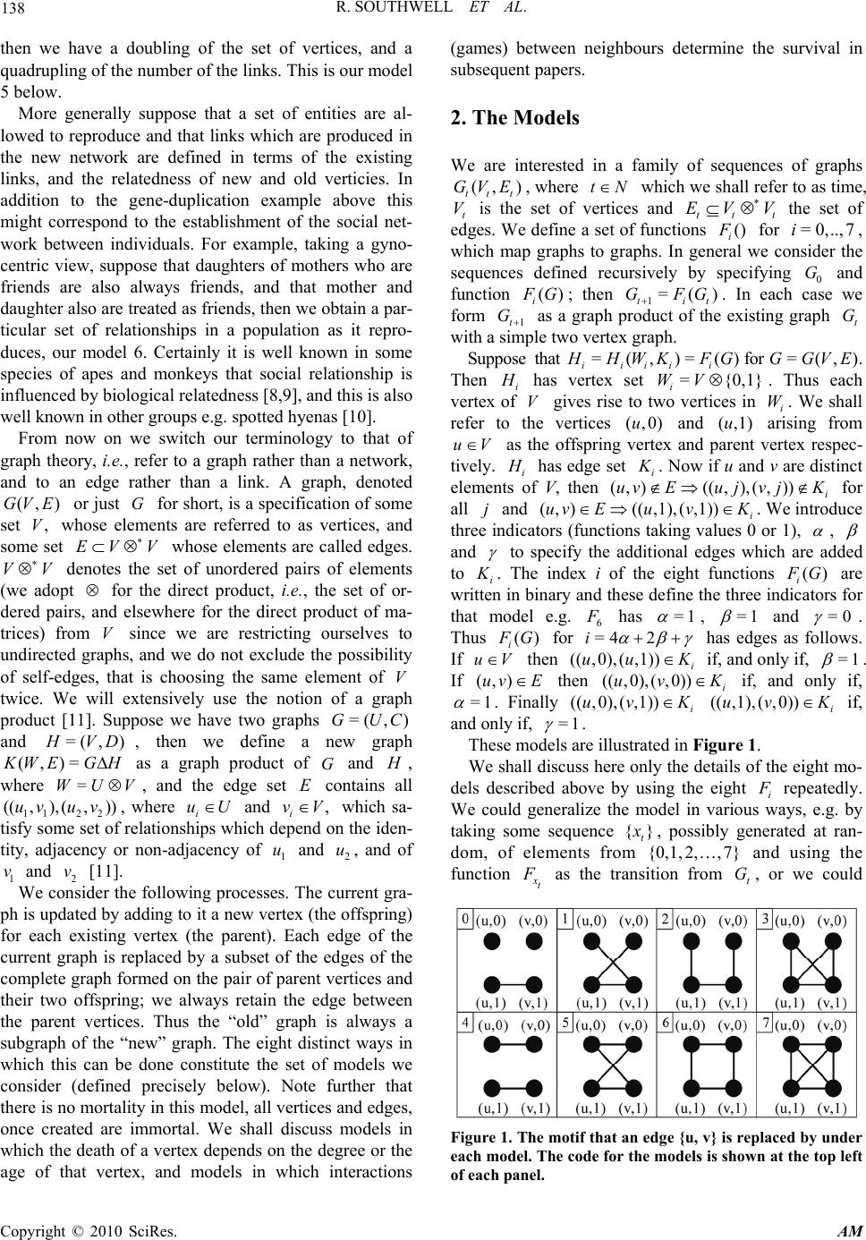

R. SOUTHWELL ET AL.
138
then we have a doubling of the set of vertices, and a
quadrupling of the number of the links. This is our model
5 below.
More generally suppose that a set of entities are al-
lowed to reproduce and that links which are produced in
the new network are defined in terms of the existing
links, and the relatedness of new and old verticies. In
addition to the gene-duplication example above this
might correspond to the establishment of the social net-
work between individuals. For example, taking a gyno-
centric view, suppose that daughters of mothers who are
friends are also always friends, and that mother and
daughter also are treated as friends, then we obtain a par-
ticular set of relationships in a population as it repro-
duces, our model 6. Certainly it is well known in some
species of apes and monkeys that social relationship is
influenced by biological relatedness [8,9], and this is also
well known in other groups e.g. spotted hyenas [10].
From now on we switch our terminology to that of
graph theory, i.e., refer to a graph rather than a network,
and to an edge rather than a link. A graph, denoted
(, )GV E or just G for short, is a specification of some
set ,V whose elements are referred to as vertices, and
some set EV V

 whose elements are called edges.
VV

 denotes the set of unordered pairs of elements
(we adopt  for the direct product, i.e., the set of or-
dered pairs, and elsewhere for the direct product of ma-
trices) from V since we are restricting ourselves to
undirected graphs, and we do not exclude the possibility
of self-edges, that is choosing the same element of V
twice. We will extensively use the notion of a graph
product [11]. Suppose we have two graphs =( , )GUC
and =( ,)
H
VD , then we define a new graph
(,)=KW EGH as a graph product of G and
H
,
where =WUV, and the edge set E contains all
112 2
(( ,),(,))uvuv, where i uU and ,
i
vV which sa-
tisfy some set of relationships which depend on the iden-
tity, adjacency or non-adjacency of 1
u and 2 u, and of
1
v and 2 v [11].
We consider the following processes. The current gra-
ph is updated by adding to it a new vertex (the offspring)
for each existing vertex (the parent). Each edge of the
current graph is replaced by a subset of the edges of the
complete graph formed on the pair of parent vertices and
their two offspring; we always retain the edge between
the parent vertices. Thus the “old” graph is always a
subgraph of the “new” graph. The eight distinct ways in
which this can be done constitute the set of models we
consider (defined precisely below). Note further that
there is no mortality in this model, all vertices and edges,
once created are immortal. We shall discuss models in
which the death of a vertex depends on the degree or the
age of that vertex, and models in which interactions
(games) between neighbours determine the survival in
subsequent papers.
2. The Models
We are interested in a family of sequences of graphs
(, )
tt t
GVE , where tN

which we shall refer to as time,
t
V is the set of vertices and tt t
EV V

 the set of
edges. We define a set of functions ()
i
F
for =0,..,7i,
which map graphs to graphs. In general we consider the
sequences defined recursively by specifying 0 G and
function ()
i
F
G; then 1=()
tit
GFG
. In each case we
form 1t G

as a graph product of the existing graph t G
with a simple two vertex graph.
Suppose that =(,)=()
iiiii
H
HWK FG for =(,)GGVE.
Then i
H
has vertex set ={0,1}
i
WV. Thus each
vertex of V gives rise to two vertices in i W. We shall
refer to the vertices (,0)u and (,1)u arising from
uV

as the offspring vertex and parent vertex respec-
tively. i
H
has edge set i K. Now if u and v are distinct
elements of V, then (,)((,),(,)) i uvEu jv jK for
all
j
and (,)((,1),(,1)) i uv EuvK

. We introduce
three indicators (functions taking values 0 or 1),

,

and

to specify the additional edges which are added
to i K. The index i of the eight functions ()
i
F
G are
written in binary and these define the three indicators for
that model e.g. 6
F
has =1

, =1

and =0

.
Thus ()
i
F
G for =4 2i



 has edges as follows.
If uV

then (( ,0),( ,1))i uu K if, and only if, =1

.
If (,)uv E

then ((,0),(,0))i uv K if, and only if,
=1

. Finally ((,0),(,1))i uv K ((,1),( ,0))i uv K if,
and only if, =1

.
These models are illustrated in Figure 1.
We shall discuss here only the details of the eight mo-
dels described above by using the eight i
F
repeatedly.
We could generalize the model in various ways, e.g. by
taking some sequence {}
t
x
, possibly generated at ran-
dom, of elements from {0,1, 2,,7} and using the
function
x
t
F
as the transition from t G, or we could
Figure 1. The motif that an edge {u, v} is replaced by under
each model. The code for the models is shown at the top left
of each panel.

R. SOUTHWELL ET AL.
139
take the

,

and

themselves to be probabilities
that the corresponding edges are included at each stage.
We shall derive results for our models for the number
of vertices with degree d, the total number of edges, the
chromatic number, diameter and average distance, and
comment briefly on the automorphisms. A further paper
will explore additional graph entities such as cliques, and
cycles, the number of polygons of given size arising
from a given polygon at the previous time step, and add
further information regarding some of the entities ex-
plored here.
As stated above the operations introduced here are all
equivalent to taking a graph product of T G with some
simple graph Z. Table 1 specifies the products for each
of the models.
3. Binary String Representation
As mentioned above, a useful, alternative way to define
the rules is in terms of the notion of parent and offspring
vertices, and binary strings. If we begin with a graph
00 0
(, )GV E, then if 0 uV, this vertex gives rise to
(,1)u and (,0)u in 1 G, which we write as u0 and u1,
and to (( ,1),1)u, ((,1),0)u ((,0),1)u and (( ,0),0)u
in 2 G, which are written in the obvious way as u11, u10,
u01 and u00, and so on. In t G there will be 2t verti-
ces arising from u. We denote these vertices as strings of
length (1)t written u

where

runs over the bin-
ary strings of length t. We refer to these representations
as vertex strings.
The eight models, all of which at time t have 0
||2
t
V

vertex strings, give rise to distinct edge sets. We now
specify precisely the edge set for each model at time t.
Consider two vertices t ux and t vy (possibly identical)
at time t, so t
x
and t
y
are two binary strings of length
t, whose I’th elements are denoted by i
t
x
and i
t
y. Now
we define a third string t z, where the i'th element of t z,
i
t
z
, is determined by the pair (, )
ii
tt
x
y. The purpose of
t
z is to specify the sequence of edges which need to be
added to u and v in order to reach t ux and t vy . In
specifying the models earlier we introduced

,

and

, as indicators for the three distinct types of new edge.
Here we identify the elements of t z with

,

,

and two new terms *

and

. Thus if we have
(, )=(0,0)
ii
tt
xy , indicating that an edge must be placed
between the offspring of the individuals 1t
ux

and
1t
vy , then we record =
i
t
z

. Similarly we track the
other edges, as is detailed below. Note for ease we in-
troduce a

corresponding to the choice (, )=(1,1)
ii
tt
xy ,
and differentiate between (, )=(0,1)
ii
tt
xy and (, )
ii
tt
x
y
=(1,0) by using

and *

respectively. When we
use the t z’s to specify which edges exist in t G, we
shall in fact take =1

always, and *
=


.
Table 1. The products are denoted by a single letter K =
Kronecker, C = Cartesian, H = Comb, S = Strong = AND, N
= non-standard.
Model α β γ Product Edges of Z
0 0 0 0 K {(1,1)}
1 0 0 1 K {(0,1), (1,1)}
2 0 1 0 H {(0,1)}
3 0 1 1 N N
4 1 0 0 K {(0,0), (1,1),}
5 1 0 1 K {(0,0), (0,1), (1,1)}
6 1 1 0 C {(0,1)}
7 1 1 1 S {(0,1)}
If
1) (, )=(0,0)
ii
tt
xy then =
i
t
z

,
2) (, )=(1,1)
ii
tt
xy then =
i
t
z

,
3) (, )=(0,1)
ii
tt
xy or (, )=(1,0)
ii
tt
xy and 11 =
tt
ux vy


then =
i
t
z

,
4) (, )=(0,1)
ii
tt
xy and 11tt ux vy

 then =
i
t
z

,
5) (, )=(1,0)
ii
tt
xy and 11tt ux vy

 then * =
i
t
z

.
The string (,)t
uvz specifies the start and the se-
quence of operations which need to take place to pro-
gress from (,)uv to (,)
tt
ux vy. As examples consider
(A) vertices ( 0010101010)u and ( 0011001110)u, then
*
10
( , )=(( ,)),uvz uu

 
and (B) ( 0011001011)u
and (0011001011)v gives rise to ((, ),).uv


Further note that t
z can contain at most one

, and
then only if =uv
.
Now we assert that t
ux and t vy are linked for a
specific model if, and only if, each of the entries in t z
(such as

,

, etc.) is equal to 1. If we start with
=uv then we obtain sequences of the form
*1
=((,)<, ><,,, >),
ktk
t
zuu  
 where the
powers of the sets <> are the direct products. Note here
that

’s in front of the

must be taken as having
value 1 in every model since they relate to the same ver-
tex. If we start with uv

then we obtain sequences
*
=((,)<,,,>)
t
t
zuv   .
There is one additional complication in the case where
we have self-edges in 0
G. We need to consider the am-
biguities which may arise if =1

and =1

, since the
former acting on a vertex, and the latter acting on a self
edge at that vertex will result in the same edge. We can
deal with this case efficiently by ensuring that any vertex
with a self-edge at any time t is only subjected to one of
the operators.
For our examples above we have that (A) requires
===1


(recall =1

and *
=


always) so

R. SOUTHWELL ET AL.
140
there is an edge only in model 7, while (B) requires only
that =1

and uv (note that in the absence of a

,
=uv would only lead to two copies of the same vertex)
so there is an edge in models 4, 5, 6 and 7.
4. Homogeneity
Definition. Merger of Two Graphs
Given two graphs (,)GU E and (,)
H
VF then we
define the merger of G and
H
as the graph
(, )
J
UVEF, and denote this by GH
Theorem
For each of the models specified above given some
00 0
(, )GV E then with 1=()
tt
GFG
 and writing in the
obvious way 0
=()
t
t
GFG
we have that,

 
0
,,
t
tuv E
GFLuv

 where (,)Luv is the graph
with vertices u and v, and one edge (,)uv .
Proof
This follows immediately from the definition of the
functions ()
i
F
G. It is clear that for any (, )GV E we
have
    
,,
iii
F
GLuvF GFLuv for each
of the possible cases 1) uV, vE and (,)uv E

,
2) ,uV vV and (,)uvE, 3) uV

and
vV, and 4) uV and vV

. Then by induction the
result follows.
In view of the theorem above much of the information
is captured by considering the case where 0
G consists
of a single edge. We consider how a single edge (and
sometimes other equally simple structures) evolve under
our models.
4.1. Models 0, 1, 4 & 5; Kronecker Products
As Table 1 shows, four of the models use the Kronecker
product, in fact those for which =0

. For such products,
which we denote by , we have ()=AG H
()()
A
GAH, where ()
A
G denotes the adjacency ma-
trix of G, and  also denotes the Kronecker product
when applied to matrices. The adjacency matrices for the
Z’s of models are 0, 1, 4 and 5, respectively,
00
01



, 01
11



, 10
01



and 11
11



.
The t th Kronecker powers of these, 22
tt
 matrices,
are easy to obtain. That for model 0 has a single 1 in the
(2,2)
tt
position, and zeroes elsewhere, model 4 gives
the identity matrix, model 5 gives a matrix of 1’s. Only
model 1 has an interesting pattern, which is essentially
the bitwise AND pattern exhibited in [12], and which is
discussed below in the Section 8.
4.2. Model 2
Model 2 is particularly simple as we have a tree structure;
we simply add a new branch at each vertex. Here we can
capture all the structure by starting with 0 G as a single
isolated vertex. There are various ways to describe the
resulting tree, and these will be explored in more detail
in a subsequent paper. For the moment we give only one
such description. Starting from a single vertex labeled u,
we obtain vertices u1 and u0 which are linked, then ver-
tices u11, u10, u01 and u00. After t steps we have a tree
with 21
t

edges on the vertices of the cube of dimen-
sion t. This tree is necessarily a spanning tree. As we
make an extra step we take the current cube, with its
spanning tree, and make a copy of the cube, join vertices
of the 1t

dimensional cube to the matching vertex in
the copy. An alternate way of expressing this is to con-
sider a t-dimensional cube with all edges present. Choose
a particular coordinate and remove all the edges from the
cube for which this coordinate is 0, then move to the
cube which has this coordinate equal to 1, and within this
cube repeat the process. At each stage one removes all
the edges of a cube, whose dimension is one smaller than
at the previous step.
4.3. Models 3, 6 and 7
Model 3 is by far the most complex and interesting of the
models. We shall discuss several aspects of this model,
along with the other models, but shall postpone a fuller
discussion to subsequent papers.
In model 6 the graph arising from a single edge after t
steps is the (1)t

-dimensional cube.
In model 7 the graph arising from a single edge after t
steps is the complete graph on 1 2t vertices.
5. Numbers of Vertices and Edges
For a general 00 0 (, )GV E we have immediately that the
number of vertices at time t is 0
||*2
t
V for all models.
The number of edges on the other hand depends on the
particular model, and can be relatively easily deduced
from the t z possibilities and the

etc. appropriate for
each model. For example, for model 3, we have
*
====1  , so for uv we have=
t
z(( , )uv
*
<,, >)
t
 so there are clearly 3t edges for each
(,)uv. We have




*1
=,<,> <,,>
ktk
t
z
uu 


and this results in (32 )
tt
 edges for each u. The com-
plete set of formulae are given in Table 2.
6. Chromatic Number
A vertex colouring of a graph G is the assignment of a
colour to each vertex in such a way that no adjacent ver-
tices in G have the same colour. The minimal number of
colours required to achieve this is the chromatic number,

R. SOUTHWELL ET AL.
141
Table 2. Formulae describing the number of edges after t
time steps within the different models.
Model Number of Edges
0 0
||E
1 0
3||
tE
2 00
(21) ||||
tVE
3 00
(32) ||3||
tt t
VE
4 0
2| |
tE
5 0
4||
tE
6 1
00
*2||2 ||
tt
tV E

7 11
00
(2 * 42)||4||
tt t
VE


which we denote by ()G  . A colouring which achieves
this minimum will be refered to as a minimal colouring.
With the exception of model 7, the chromatic number of
the growing graphs are easy to obtain.
6.1. Models 0, 1, 4 and 5
Suppose that we have a minimal colouring for 0 G with
0
()G  colours. For models 0, 1, 4 and 5, each offspring
can be given the same colour as its parent without vio-
lating the condition that we have a colouring, and so the
chromatic number remains equal to 0 ()G  .
6.2. Models 2 and 6
For models 2 and 6, suppose we have a minimal colour-
ing of 0
G using the set 01 ()1
0
{,, ,}
G
cc c
 
 of 0
()G 
colours. Now suppose that the offspring of a vertex col-
oured with i
c is coloured (1)( )
0
imodG
c
 . Then, provided
0
()>1G  this will constitute a minimal colouring for
0
()
i
RG for =2i and for =6i. Thus






0
=2,
t
Gmax G  .
6.3. Model 3
In this model 1 ()=()1
tt
GG 


. This is because in any
minimal, proper colouring of t G there will be an indi-
vidual with ()1
t
G   distinct colours amongst its
neighbours (actually there will be at least ()
t
G  such
individuals, and since this individual's offspring is joined
both to the individual and all its neighbours, this off-
spring must be given a new colour. This colour can then
be given to every offspring.
6.4. Model 7
This is by far the most difficult case, and will be treated
more fully elsewhere. We observe only that
()1 ()2()
ttt
GGG   .
The first inequality follows since model 3 produces a
subgraph of model 7 when they act on the same G. The
latter inequality is evident since giving a minimal, proper
colouring of t
G using colours 01 ()1
0
{,, ,}
G
cc c
 
 we
can colour the offspring of any vertex coloured i
c with
some i
c

, from a set ** *
01 ()1
0
{, ,,}
G
cc c
 
 of completely
new colours. It is clear that if t G is a clique, or bipartite,
then the chromatic number doubles, but this doubling is
not general. For example the chromatic number of any
polygonal graph Q of odd degree > 3 is 3, while
7
(())=5FQ  .
7. The Distance Structure
We now turn to the details of the distances between ver-
tices. The distance between vertices u and v is denoted
by (,)duv, the diameter of a graph g by ()G
 . For a
graph t
G we denote the numbers of pairs of vertices
with distance x as ()
t
x
 . For each models we shall de-
rive the recursions for the distances through time. Mod-
els 0 and 4 are excluded since they lead to disconnected
components for which the notion of distance is inappro-
priate. We also suppose that our initial graph is con-
nected so that all subsequent graphs are.
7.1. Model 2
We begin with model 2 since this will allow an easy de-
monstration of our methods. It is clear that
1
()=( )2
tt
GG 


. As in every model if t uV

then
(0,1)=1du u, while if (,) t uv E with (,)=duv d
then
(1,1)=du vd, (1, 0)=(1, 0)=1du vdu vd and
(0,0)= 2du vd

. We can then write
1(0) = 2(0) tt

,
1(1)=(0)(1) ttt

,
1(2) = 2(1)(2) ttt

 and
1()=(2)2 (1)() ttt t
kkkk  
 if 3k.
This enables us to derive closed form expressions for
the ()
ti
 , for example
0
(0) = 2(0)
t
t
 ,
00
(1) =(1)(21)(0)
t
t
   ,
and
00 0
(2) =(2)2(1)2(21)(0)
t
ttt

  
but the forms
rapidly become somewhat unmanageable.

R. SOUTHWELL ET AL.
142
We can specify the total number of distances, for all
models, 2
00
=(4||2 ||)/2
tt
t
LV V being simply the
number of pairs of vertices plus the number of vertices,
and being the same for all the models. The total of the
distances



 

**
111
2
*21 121
00 0
=443 0
=420220 .
ttt t
tt tt
LL L
Lt






The average distance *
=/
ttt
dLL
and for t large this
gives t
dct where *2
00 0
=(2(0)) / ((0))cL  . The
average distance thus increases by 1 at each stage.
We can derive this average result in another, more di-
rect way. Suppose at some stage we have n vertices and
average distance t

. Now we add the extra offspring.
The average distance is just the distance between a ran-
domly selected pair of vertices. We consider the possible
pairs in the new graph. There are (2 1)nn such pairs,
n are of type (0,1)uu and contribute a distance 1. Of
the remaining 2
2,n 1/4 are of type (1,1)uv , 1/2 are of
type (1,0)uv , and 1/4 are of type (0,0)uv , which con-
tribute (1,1),duv (1,1) 1du v

and (1,1) 2du v

re-
spectively. The average over these 2
2n latter will thus
be 1
t
  and overall we will therefore have

 
2
1
21
==1221
21
t
tt
nn nn
nn





.
A similar argument can be used to obtain an expres-
sion for the variance of the distances which asymptoti-
cally increases by 1/2 per time step.
7.2. Model 1
In order to derive the appropriate expressions for model
1 we need to track not only the distances but also the
number of edges which belong to triangles. Accordingly
we define set ()G of the edges which belong to a tri-
angle (an edge (,)uvE belongs to a triangle if there
exists some k such that (,)ik E

and (, )
j
kE). De-
fine (1)=|()|
tG

 and *(1)=(1)()
ttt
t 

. The
necessity of considering triangles arises because the off-
spring of two linked parents will be distance 3 apart if
the parents’ link is not part of a triangle, but only 2 apart
if there is a triangle since they are linked through the
common neighbour of their parents.
In detail we have
For all uV we have (0,1)=2duu,
and for (,)uvE,
if (,)>1duv we have
(0, 0)=(0,1)=(1,0)=(1,1)=(, )duvduvdu vdu vduv,
if (,)( )uv G then (0,0)=2,du v(0,1)=du v
(1, 0)=1du v, (0,1) ()uv G and (1, 0)()uv G ,
and
if (,)\( )uv VG then (0,0)=3du v, (0,1)=du v
(1, 0)=1du v, (0,1)()uv G and (1,0)()uv G .
We have immediately that
1
()= ((),3)= ((),3)
tt
Gmax Gmax G  
.
From these expressions we obtain recursions for the

’s, as follows,
1
(0) =2(0)
tt

,
1
(1) = 3(1)
tt



**
1
(1) = 3(1)
tt


11
(2) =(0)(1)4(2)
tt tt
 



*
11
(3) =(1)4(3)
tt t



1
()=4 ()
tt
kk 
 if >3k.
From the above recursions we can find simple closed
form expressions for the

’s, as follows,
0
(0) =2(0)
t
t
 ,
0
(1) = 3(1)
t
t


**
0
(1) = 3(1)
t
t

000
(2)=(42)(0)/ 2(43)(1)4(2)
ttttt
t
 


*
00
(3) =(43)(1)4(3)
tt t
t
 
1
()=4 ()
tt
kk 
 if >3k.
The total distance
** *
000 0
= 4(43 )(2(1)(1))(42)(0)
ttttt
t
LL  

 ,
so that the average distance converges to a constant. The
variance of the distances also converges to a constant.
7.3. Model 3
We obtain, in a straightforward manner that
1
(0) =2(0)
tt

,
11
(1) =(0)3(1)
tt t


,
11
(2) =(1)4(2)
ttt


,
1
()=4 ()
tt
kk 
 for >2k.
We have
1
()= ((),2)=((),2)
tt
GmaxG maxG  
,
and the total distance
**
00 00 0
=4((0) (1))3((0) (1))
tt
t
LL     so that
the average distance converges to a constant. The vari-
ance of the distances also converges to a constant.
7.4. Model 5
We obtain 1 (0) =2(0)
tt

,
1
(1) =4(1)
tt

,
11
(2) =(0)4(2)
ttt


,
1
()=4 ()
tt
kk 
 for >2k.
We have
()=()
t
GG  ,
and the total distance
**
00 0
=4((0)) 2(0)
tt
t
LL   so that the average dis-
tance converges to a constant. The variance of the dis-
tances also converges to a constant.

R. SOUTHWELL ET AL.
143
7.5. Model 6
We obtain 1 (0) = 2(0)
tt

,
11
(1) =(0)2(1)
ttt


,
11
()=2(1) 2()
tt t
kk k  

 for 2k.
We have
1
()=( )1
tt
GG 
, and
**
111
=4 2(0)
tt tt
LL L 

 , from which we can easily
demonstrate that the average distance */
tt
L
L increases
by 1/2 per time step for large t. The variance of the dis-
tances increases by 1/4 per time step for large t.
7.6. Model 7
We obtain
1
(0) =2(0)
tt

,
11
(1) =(0)4(1)
ttt


,
1
()=4 ()
tt
kk 
 for 2k.
From this we have that the diameter is constant, and
**
00
=4(42)(0)/ 2
tt
tt
LL   ,
so the average distance converges to a constant. The
variance of the distances also converges to a constant.
8. Automorphism
In models 0, 1, 4 and 5 we have Kronecker products and
this allows us to determine the automorphisms on verti-
ces in t G. In these models for a pair of vertices ur and
vs , where u and v belong to 0 G, and r and s are binary
strings, to be automorphic in t
G, they must have u and v
automorphic in 0 G and r and s to be automorphic in the
Kronecker product of the appropriate .
Z
This is
straightforward in each of the models. The most inter-
esting case is model 1. For this the adjacency matrix is
01
=.
11
A


The n th Kronecker product, k
A
, of this matrix have
its rows and columns naturally indexed by the n th
Kronecker products of vectors (0,1) and (0,1 )T, and
will have a zero wherever the row index and column
index have a 0 in the same position. It immediately fol-
lows that the matrix k
A
is invariant under any permuta-
tion to the elements of the row and column indices. Ac-
cordingly the permutations induce an equivalence rela-
tion over the binary strings; two strings being automor-
phic if they contain the same number of 0’s.
9. Generating All Graphs
Now [4] proved that for any graph (,)
H
UF of order n
there exists a set W of size 2/4n such that one can
associate distinct subsets i W with the n vertices, such
that (, )ij F

if, and only if, =
ij
WW

. Consider
the case where we evolve a single vertex, linked to itself,
for t time steps under model 1. The vertex set of the re-
sulting graph will be the set of t length binary strings.
Suppose each string t
x
is associated with a set
()={| =0}
i
tt
Sxi x. Then two vertices, t
x
and t
y
, are
joined if, and only, () ()=
tt
Sx Sy

. It follows that
every graph with n vertices is isomorphic to some sub-
graph of the t’th iterate when 2/4tn

 .
Now as pointed out in [4] the bound is exact only
when the graph H is bipartite with vertices partitioned
equally, when n is even, and differing by 1 when n is odd.
Thus we will observe many graphs will appear at earlier
stages, for example the graph n K, the complete graph
on n vertices, will appear at time =1tn, since we
may take ={}
i
Wi. We shall investigate this phenome-
non elsewhere.
10. The Degree Distribution
Since we have a deterministic process the degrees of the
vertices are well defined. We denote by (,)DGx the
number of vertices of degree x in graph G, and refer to
the degree of any vertex x as ()deg x. We shall refer to
the degree distribution by which we mean the distribu-
tion of the degree of a randomly chosen vertex.
10.1. Degree Distribution; Models 0, 1, 4, 5
We begin with the models which are Kronecker products.
Given two graphs =( ,)
J
VE and =( , )KWF with
yV

with ()deg y and zW with ()deg z, then for
(,)
y
zJK

 we have ((,))=()*degy zdegy()deg z.
It follows that


()
,=, ,
ji
D
JKx DJjDKij
 

where ()={|,| }ijjNji  , |
j
i having the usual
meaning that j divides i.
Now in these models we have 0 =
tt
GG Z, where
t
Z
is the graph obtained by taking the graph
Z
(as
described in Table 1) and taking the Kronecker product
of it with itself t times. By knowing the degree distribu-
tion of t
Z
one can easily determine the distribution
starting from a generic initial graph. Under model 0, t
Z
has (2 1)
t

isolated vertices and a single vertex with
degree 1, model 1 has tr C vertices with degree 2r,
model 4 has every vertex with degree 1, while model 5
has every vertex with degree 2t.
10.2. Degree Distribution; Model 2
At each stage all the vertices of t G increase their de-

R. SOUTHWELL ET AL.
144
gree by 1, and a set of ||
t
G vertices of degree 1 are
added. Thus 0
=0
(,)=( )(,)
t
ttr
r
D
GxCDGx r
.
10.3. Degree Distribution; Model 6
For model 6 we have a Cartesian product (which we de-
note ). For graphs =( ,)
J
VE and =( , )KWF with
yV with ()deg y and zW with ()deg z, then for
(,)
y
zJK we have ((,)=()()degy zdegydegz.
Thus
 
0
,,,
i
j
DJ KxDJjDKij




and since the Cartesian power ({0,1}, (0,1))
tG is sim-
ply the t dimensional cube we have that




0
,=2 ,
t
t
D
GxDGx t.
10.4. Degree Distribution; Models 3 and 7
As usual model 3 is the most interesting, and the most
difficult model to deal with. A vertex t vG with de-
gree x gives rise to 1v with degree 21
x
 and to 0v
with degree 1
x
. Thus
11
(,)=(,1)(,(1)/2
tt t
DG xDGxDGx


A plot of the frequency distribution of degrees for t = 17
is shown in Figure 2.
This distribution will be explored further in subse-
quent papers.
In model 7 a vertex t vG with degree x gives rise to
two vertices, 1v and 0v, each with degree 21
x

. If
follows that





0
,=2, 122
ttt
t
DG xDGx
11. Discussion
We have presented a variety of models for the growth of
networks based on parent-offspring links and suggested
that these might be used to describe the growth of inter-
actions between individuals within a population.
This description might well be used to represent the bin-
ding of proteins under gene- and or genome-duplications.
Alternately we might be describing the interactions within
a population of organisms where these interactions de-
pend on the interactions which existed amongst those in
the previous generation, such as dominance relations
(though these might require a directed graph approach).
The model as formulated has deliberately been kept as
simple as possible. Thus the model is deterministic. The
deterministic assumption would rarely apply in a bio-
logical context, but might in a computer context. We
Figure 2. A truncated plot showing the frequencies of ver-
tices with degree ≤ 5000 within the graph obtained by
evolving a single edge for 17 time steps under model 3.
have indicated some ways in which a stochastic element
can be introduced. One can vary the transition function
applied as a stochastic process, or one can vary the links
made by making the parameters of the models probabili-
ties, rather than 0 or 1.
The simplicity of our model has allowed us to derive
many results. Perhaps the most important of these is the
theorem from Section 4. This theorem highlights the fact
that the growth of any subgraph is independent of the
nature of its exterior surroundings. By using this result
and exploiting relations with graph products and binary
strings we have derived formulas that describe chromatic
number, distance structure and degree distributions.
The model has immortal vertices and edges. In subse-
quent papers we shall consider models with a similar
reproductive structure, but allow for the death of vertices.
In the next paper we shall treat the case where individu-
als have a fixed lifetime, and in the third we shall apply a
threshold to the degree of a vertex, nodes which accu-
mulate too high a degree will die. Naturally both of these
processes could be made stochastic. In these models
edges, once established through the reproductive phase
disappear solely because of the death of one of their ver-
tices. Additional features which we shall add in the fu-
ture include sexual reproduction, and the embedding of
the graph in space.

R. SOUTHWELL ET AL.
145
12. Acknowledgements
The authors gratefully acknowledge support from the
EPSRC (Grant EP/D003105/1) and helpful input from Dr
Jonathan Jordan, and others in the Amorph Research
Project (www.amorph.group.shef.ac.uk).
13. References
[1] G. U. Yule, “A Mathematical Theory of Evolution, Based
on the Conclusions of Dr. J. C. Willis, F.R.S.,” Philoso-
phical Transactions of the Royal Society of London (Se-
ries B), Vol. 213, 1925, pp. 21-87.
[2] H. A. Simon, “On a Class of Skew Distribution Func-
tions,” Biometrika, Vol. 42, No. 3-4, 1955, pp. 425-440.
[3] A. L. Barab´asi and R. Albert, “Emergence of Scaling in
Random Networks,” Science, Vol. 286, No. 5439, 1999,
pp. 509-512.
[4] B. Bollob’as, O. Riordan and G. Spenser, “The Degree
Sequence of a Scale-Free Random Graph,” Random
Structures and Algorithms, Vol. 18, No. 3, 2001, pp. 279-
290.
[5] J. Jordan, “The Degree Sequences and Spectra of
Scale-Free Random Graphs,” Random Structures and
Algorithms, Vol. 29, No. 2, 2006, pp. 226-242.
[6] C. Cannings and A. W. Thomas, “Handbook of Statistical
Genetics,” John Wiley and Sons Ltd, New York, 2007.
[7] J. S. Taylor and J. Raes, “Duplication and Divergence:
The Evolution of New Genes and Old Ideas,” Annual Re-
view of Genetics, Vol. 38, No. 1, 2004, pp. 615-643.
[8] A. Widdig, P. Nurnberg, M. Krawczak, W. J. Streich and
F. B. Bercovitch, “Paternal Relatedness and Age Prox-
imity Regulate Social Relationships among Adult Female
Rhesus Macaques,” Proceedings of the National Acad-
emy of Science USA, Vol. 98, No. 24, 2001, pp. 13769-
13773.
[9] G. Hausfater, “Dominance and Reproduction in Baboons
(Papio Cynocephalus),” Contributions to Primatology,
Vol. 7, 1975, pp. 1-150.
[10] L. Frank, K. Holekamp and L. Smale, “Serengeti II: Dy-
namics, Management, and Conservation of an Ecosys-
tem,” University of Chicago Press, Chicago, 1995.
[11] W. Imrich and S. Klavar, “Product Graphs: Structure and
Recognition,” John Wiley and Sons Ltd, New York,
2000.
[12] S. Wolfram, “A New Kind of Science,” Wolfram Media,
Inc., Champaign, 2002.
[13] P. Erd¨os, A. W. Goodman and L. Posa, “The Represen-
tation of a Graph by Set Intersections,” Canadian Journal
of Mathematics, Vol. 18, No. 1, 1966, pp. 106-112.