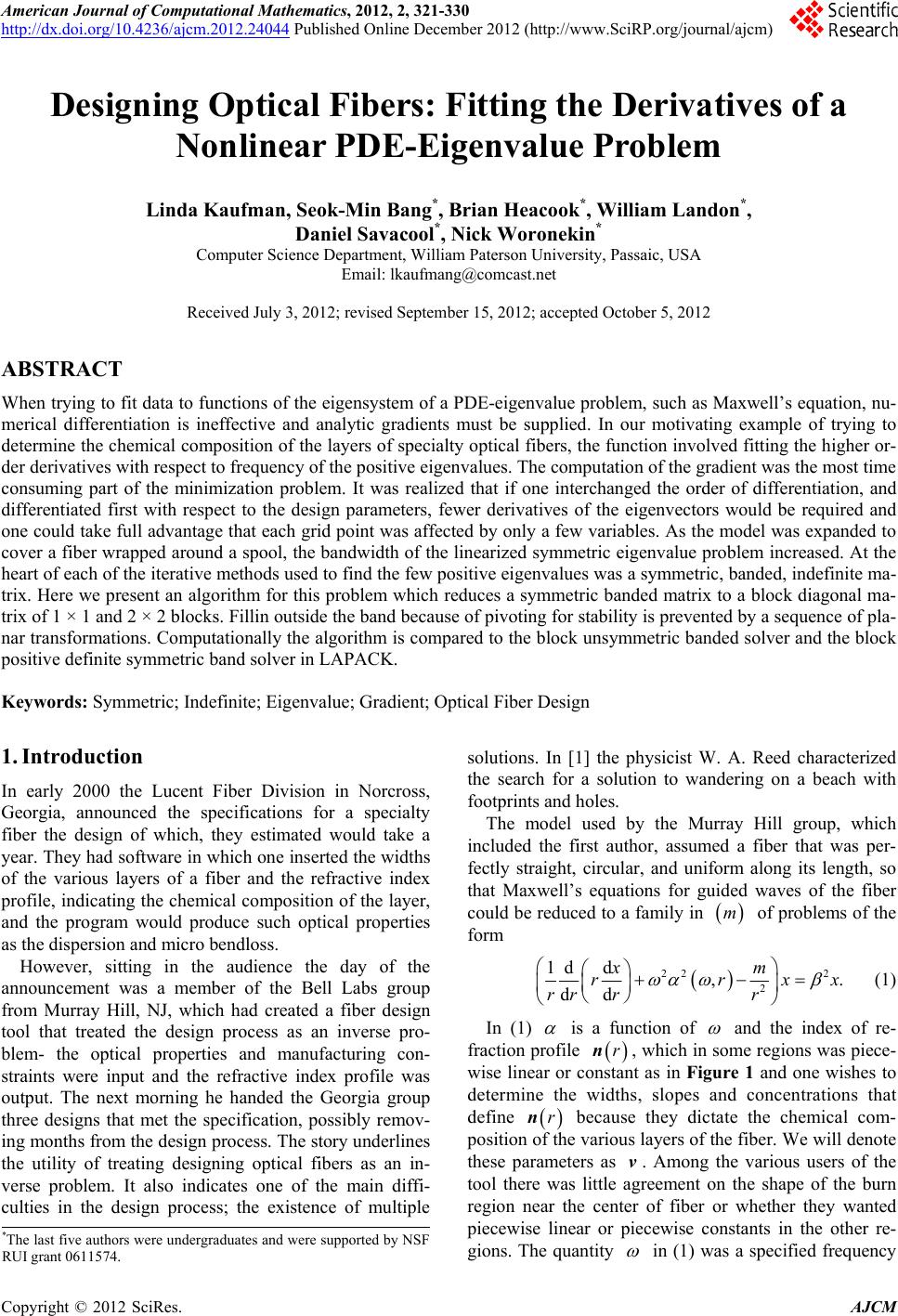
American Journal of Computational Mathematics, 2012, 2, 321-330
http://dx.doi.org/10.4236/ajcm.2012.24044 Published Online December 2012 (http://www.SciRP.org/journal/ajcm)
Designing Optical Fibers: Fitting the Derivatives of a
Nonlinear PDE-Eigenvalue Problem
Linda Kaufman, Seok-Min Bang*, Brian Heacook*, William Landon*,
Daniel Savacool*, Nick Woronekin*
Computer Science Department, William Paterson University, Passaic, USA
Received July 3, 2012; revised September 15, 2012; accepted October 5, 2012
ABSTRACT
When trying to fit data to functions of the eigensystem of a PDE-eigenvalue problem, such as Maxwell’s equation, nu-
merical differentiation is ineffective and analytic gradients must be supplied. In our motivating example of trying to
determine the chemical composition of the layers of specialty optical fibers, the function involved fitting the higher or-
der derivatives with respect to frequency of the positive eigenvalues. The computation of the gradient was the most time
consuming part of the minimization problem. It was realized that if one interchanged the order of differentiation, and
differentiated first with respect to the design parameters, fewer derivatives of the eigenvectors would be required and
one could take full advantage that each grid point was affected by only a few variables. As the model was expanded to
cover a fiber wrapped around a spool, the bandwidth of the linearized symmetric eigenvalue problem increased. At the
heart of each of the iterative methods used to find the few positive eigenvalues was a symmetric, banded, indefinite ma-
trix. Here we present an algorithm for this problem which reduces a symmetric banded matrix to a block diagonal ma-
trix of 1 × 1 and 2 × 2 blocks. Fillin outside the band because of pivoting for stability is prevented by a sequence of pla-
nar transformations. Computationally the algorithm is compared to the block unsymmetric banded solver and the block
positive definite symmetric band solver in LAPACK.
Keywords: Symmetric; Indefinite; Eigenvalue; Gradient; Optical Fiber Design
1. Introduction
In early 2000 the Lucent Fiber Division in Norcross,
Georgia, announced the specifications for a specialty
fiber the design of which, they estimated would take a
year. They had software in which one inserted the widths
of the various layers of a fiber and the refractive index
profile, indicating the chemical composition of the layer,
and the program would produce such optical properties
as the dispersion and micro bendloss.
However, sitting in the audience the day of the
announcement was a member of the Bell Labs group
from Murray Hill, NJ, which had created a fiber design
tool that treated the design process as an inverse pro-
blem- the optical properties and manufacturing con-
straints were input and the refractive index profile was
output. The next morning he handed the Georgia group
three designs that met the specification, possibly remov-
ing months from the design process. The story underlines
the utility of treating designing optical fibers as an in-
verse problem. It also indicates one of the main diffi-
culties in the design process; the existence of multiple
solutions. In [1] the physicist W. A. Reed characterized
the search for a solution to wandering on a beach with
footprints and holes.
The model used by the Murray Hill group, which
included the first author, assumed a fiber that was per-
fectly straight, circular, and uniform along its length, so
that Maxwell’s equations for guided waves of the fiber
could be reduced to a family in of problems of the
form

m

22 2
2
1d d,.
dd
xm
rrx
rr rrx

 



 


(1)
In (1)

is a function of

and the index of re-
fraction profile


rn, which in some regions was piece-
wise linear or constant as in Figure 1 and one wishes to
determine the widths, slopes and concentrations that
define


rn because they dictate the chemical com-
position of the various layers of the fiber. We will denote
these parameters as . Among the various users of the
tool there was little agreement on the shape of the burn
region near the center of fiber or whether they wanted
piecewise linear or piecewise constants in the other re-
gions. The quantity
v

in (1) was a specified frequency
*The last five authors were undergraduates and were supported by NSF
RUI grant 0611574.
C
opyright © 2012 SciRes. AJCM

L. KAUFMAN ET AL. 322
Figure 1. A typical index profile with parameters.
and m was a specified mode number. For a typical
problem there might be about 20 values of

and
might take on integer values between 0 and 2.
m
According to the Modified Chemical Vapor Deposi-
tion (MCVD) technique, a hollow cylinder several feet
long and several inches in radius is put on a lathe and
gases such as silicon dioxide, gallium and fluourine are
introduced into this tube, according to the specification
of the refractive index profile in , and these gases
deposit themselves on the interior of the cylinder until it
is solid. The cylinder or preform is then put in a draw
tower, its end is heated, and the fiber is drawn to the
specified width. The modeling process here assumes that
the chemicals on a given cross section of the preform
will be found in the same arrangement on the fiber.

rn
The waveform in (1) is truncated at some radius
beyond the core of the fiber and the boundary condition
is expressed as the order modified Bessel function
of the second kind [2]. A finite element approach can be
used to approximate (1) and converts the family of
differential equations in (1) to a family of symmetric
generalized tridiagonal eigenvalue problems
th
m


T.
qq
As

ee xx (2)
where

s

involves Bessel functions, A is a q × q
symmetric tridiagonal matrix for a finite element discreti-
zation, q is the last column of the q × q Identity matrix,
and M is the diagonal positive definite mass matrix
which represents the inner product of the basis functions
used in the finite element method. Thus the boundary
condition changes the problem from finding the positive
eigenvalues and corresponding eigenvectors of about 60
linear eigenvalue problems to 60 nonlinear eigenvalue
problems per function evaluation.
e
Although solving the nonlinear eigenvalue problem is
essential to designing the fiber, it is not the complete
story. Depending on the ultimate use of the fiber (local
area network, underwater transmissions, or to splice into
an existing network to restore a degraded signal), after
the appropriate eigenvalues and eigenvectors are deter-
mined, as explained in [3], a user might wish to evaluate
the dispersion given by
2
,





 (3)
the dispersion slope,
3
2,





 (4)
where

is the wavelength and 2πc

  where the
frequency

is measured in radians per second and
is the speed of light, the effective area given by
c
2
4
d
2π,
d
x
rr
x
rr

 (5)
the Laplace Spot Size or the square of the second Peter-
man Radius given by
2
2
d
2
dd
d
x
rr
xrr
r





, the microbend loss,
which depends on the Laplace Spot size and the RMS
Spot size =
12
3
2
d
2d
x
rr
x
rr







, the macrobendloss, or the
cutoff ratio, the largest value of

, for which there are
no positive eigenvalues.
The design problem can thus be posed as a constrained
nonlinear least squares problem of trying to meet target
values of say the dispersion (3) and/or the effective area
(5) for values of

while keeping the width of regions
nonnegative and satisfying manufacturing constraints.
Because of the complexity of the eigenvalue computation
and the further construction of the optical properties,
optimizers tend to balk with numerical differentiation.
There are many tantalizing aspects of this problem in-
cluding the determination of an appropriate grid which
couild change as the width parameters of the layers
changed, the solution of the nonlinear eigenvalue pro-
blem, and the characterization of the nature of the mul-
tiple solutions of the inverse problem. In this paper we
will concentrate on some of the ideas that were not incor-
porated in the original package but were developed when
the first author moved to academia and was no longer in
the mode of trying to meet the immediate demands of
customers.
Often the solution of the eigenvalue problem required
only about 20 to 30 percent of the computation time.
Calculating the quantities in (3)-(5) and their derivatives
with respect to the design parameters took up most of the
remainder of the time. Initially one should always use
symbolic and/or automatic differentiators like ADIFOR
[4] to make sure that the derivative are correct, but

L. KAUFMAN ET AL. 323
we found that using these techniques we were spend- ing
much time computing quantities that were zero. In
Section 2 we consider ways to reduce the computation
cost of the derivatives. These techniques were suitable
for undergraduates like the last 5 authors and hopefully
these techniques might have more general application in
other inverse problems. Specifically, we were concerned
about whether it was best to interchange the order of
differentiation if part of the objective function was a
derivative as in (3), whether it paid to use the fact that for
certain parameters, like the heights of the layers, the
matrix
p
A
was only nonzero in the portion of its rows
corresponding to the grid points of the current layer, and
thirdly, how could one take advantage of the fact one
could write the original matrix A as a linear combination
of vectors where the coefficients were dependent only on

and the vectors were dependent only on


rn—i.e.
the variables separated.
Solving the fiber optics problem was not a one way
street of technology transfer and hopefully this paper will
serve to highlight some of the linear algebraic advances
that were stimulated by this application. Several non-
linear eigensolvers that were applied to the problem were
compared in [5], which in turn partly motivated the re-
search in [6-10]. Each of these solvers required the
solution of many symmetric indefinite tridiagonal sys-
tems. Augmenting the simple model in (1) to handle a
fiber wrapped around a spool, changed the tridiagonal
eigenvalue problem to a 7-diagonal eigenvalue problem
with the largest elements on the main diagonal and the
outermost diagonal. In [11], algorithms for solving sym-
metric indefinite banded tridiagonal and 5 diagonal sy-
stems are given. If the number of diagonals exceeds 5,
the bandwidth could increase especially if the largest
elements appeared on the outermost diagonal. The appli-
cation motivated the first author of this paper, who was
also a coauthor of [11] to investigate further the larger
bandwidth problem. In Section 3 we discuss an algorithm
for solving the symmetric indefinite banded system with
bandwidths larger than 5 that was initially given in [12]
and indicate how one can form a block version of the
algorithm.
2. Obtaining Analytic Derivatives
In this section we look at techniques that can be used to
speed up the computation of the derivatives. Table 1
gives the percentage of the computation time used to
solve the eigenvalue problem (1) and then to compute the
various quantities like the dispersion slope (4) and the
effective area and their derivatives with respect to the 12
design parameters. In general each run involved about
solving about 1800 eigenvalue systems assuming 30 fun-
ction and/or gradient evaluations per run: Each function
evaluation required finding the positive eigenvalues and
their corresponding eigenvectors of about 60 systems for
about 20 values of

and 3 of m. The point of the table
is that an efficient eigensolver only tackles some of the
problem.
To get derivatives one can augment the system of
differential equations to obtain the derivatives with re-
spect to the design parameters but this would increase the
dimension of the eigenvalue problem. A better idea
would be to move immediately into the discrete domain.
According to [2], if one uses a finite element method
with a spacing

, then the eigenvalue

of (2) satis-
fies 22
cl
2
 k 

 where

is defined in (1) and
cl is the wave number of the cladding. In general the
wave number is given by
k
c

n.
To simplify our notation let

T.
qq
BAs   ee (6)
and let be
p

or one of the design parameters in v
used in defining n. Modifying the classical formulation
for the classical formulation for the derivative of the
eigenvalues found in [13], and differentiating
BM


xx, we get
 
T
qq
MA sMB
pp




p


 




x
ee x (7)
which when multiplied by eliminates the right hand
side of (7) giving
T
x


TT
,
qq
s
AM
pp p p






 

  
xeex
(8)
where 2
1q
s
x

  , if one stipulates that T1M

xx .
The formula given in (8) is basic to approximating the
function value and some of the gradient of the function.
The major part of the computation of the dispersion and
dispersion slope required the second and third derivatives
of

with respect of

. If we let

 denote the
derivative of

with respect to

, and
A

the
derivative of A with respect to

, then if we
differentiate (2) twice with respect to

, multiply the
result by and use the fact that we get the
following formula to be used in the calculation of the
dispersion:
T
x0M


TT
2,AB


 
xxxx (9)
where 22
q
s
x



, which calls for the determination
of

x, which can be determined by differentiating (2)
yielding

 
=.MB MB 

xx (10)
and using the fact that .
T0M
xx
The quantity


 required by the dispersion slope =
3
2





 can be derived similarly and is given by

L. KAUFMAN ET AL. 324
Table 1. Percentage of time spent in various operations with
12 variables.
Operation Function only Derivatives also
Building A, M and their derivatives 5 16
Solving the eigenvalue problem 84 27
Derivatives of the eigensystem 0 10
Dispersion and slope 7 36
Effective area and Peterman radii 3 12

TT TT
333ABBM




  
 xxxxxx xx(11)
where the quantity

has all the terms in


2
q
xs



except 2
q
s
x


 .
2.1. Interchanging the Order of Differentiation
Now let us consider formulae for the derivatives of (9)
and (11) with respect to a parameter .
p
If one uses the convention that
p
A
is the derivative
of the A matrix with respect to the pth parameter and
p
x
is the derivative of the eigenvector with respect to
the design parameter , then it has been shown in [14]
that if
x
th
p

contains all the known terms in

p
s2




then
p

 can be expressed several ways including

 
T
TTTT
2
pp
p
A
BBBB



 



ppp
xx
x x xxxx xx
(12)
where

collects the terms other than

2
pq
x
s


 in

2
qp
xs


 and 
p
x satisfies


p
p
MB MB
MB MB






 
p
p
xx
xx
TT
and the condition
M
M


p
p
xxx x
xx
. Table 1 uses the
formula in (12) which requires , , and for the
design parameter
th
p
p
x and

p
x. For 12 design parame-
ters one must solve for 26 vectors.
Another formula for the gradient vector of the dis-
persion can be derived by interchanging the order of
differentiation. More specifically, one begins with (7) for
the design parameter, multiplies through by to
remove the term with the derivative of the vector and
then continues to differentiate with respect to
th
pT x

yield-
ing the equation



where



2
,
MB MB
MB





 


xx
x

(14)
and TT
M
M

 xxx x 
.
The second formula for
p

 in (13) requires , x

x,


x. Thus for 12 design parameters the formula in (13)
requires 3 vectors. Theoretically, (12) requires at least
twice as much work as (13).
The gradient of the dispersion slope (4) with respect to
the design parameter requires the derivative of
th
p



with respect to that parameter. We have looked at several
formulae for
p


 including




TTT
TT TT
TT T
TT T
2
3
333
3
ppp p
p
ppp
pp
AMB
BB BB
BB M
MM M





 
 



 

 

pp
p
xxx xxx
xxxxxxxx
xx xxxx
xxx xxx
p
(15)
where

has all terms in except


2
qp
xs 




2
pq
x
s


 and




TTT
T
TT
TT
TTT T
2
2
6(
.
ppp p
p
pp
pp
pppp
AMB
M
MM
MM
BBB B






 
 
 



  
 
xxx xxx
xx
xxx x
xxx x
xxxxxxxx
(16)

TT T
TT
TTT
42
2
42
p
pp p
pp
ppp
AB B
BM
MMM


.



   
 

 
 
xxxxxx
xxx x
xxx xxx
The main advantage of (16) is that one does not have
to compute
p
x,

p
x, and 
p
x, which are the most time
consuming portions of (15). It was derived by first diffe-
rentiating with respect to the design parameter and then
with respect to ω three times. From Table 2 we see the
advantage of using (16) and (13) over (15) and (12) just
by changing the formulae. Using both sets of formulae
the numerical values for the gradient of the dispersion
and its slope are the same as long as the eigenvalues are
accurate to full precision. Although
p
x is not needed in
(16), it is needed to compute the gradient of the effective
area if that is part of the specifications of the fiber.

(13) The theory and methodology given in (15) for (1) can
be easily extended to spooled models or full vector
models and other approximations of the differential
operator such as those used in [15,16], or the plane-wave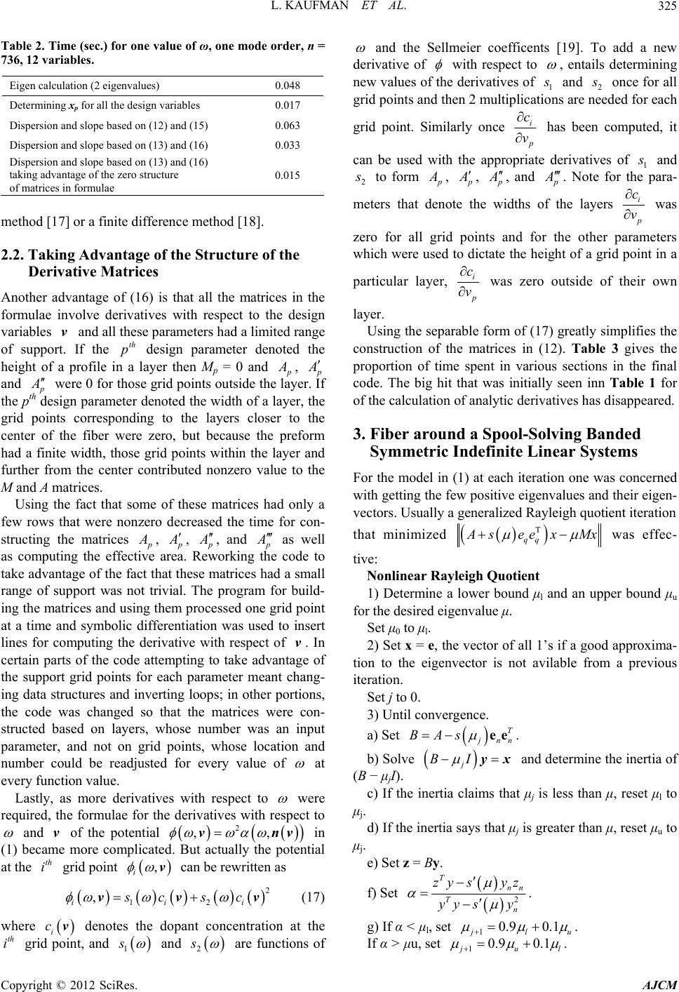

L. KAUFMAN ET AL. 325
Table 2. Time (sec.) for one value of ω, one mode order, n =
736, 12 variables.
Eigen calculation (2 eigenvalues) 0.048
Determining xp for all the design variables 0.017
Dispersion and slope based on (12) and (15) 0.063
Dispersion and slope based on (13) and (16) 0.033
Dispersion and slope based on (13) and (16)
taking advantage of the zero structure
of matrices in formulae
0.015
method [17] or a finite difference method [18].
2.2. Taking Advantage of the Structure of the
Derivative Matrices
Another advantage of (16) is that all the matrices in the
formulae involve derivatives with respect to the design
variables and all these parameters had a limited range
of support. If the design parameter denoted the
height of a profile in a layer then Mp = 0 and
v
th
p
p
A
,
p
A

and
p
A
 were 0 for those grid points outside the layer. If
the pth design parameter denoted the width of a layer, the
grid points corresponding to the layers closer to the
center of the fiber were zero, but because the preform
had a finite width, those grid points within the layer and
further from the center contributed nonzero value to the
M and A matrices.
Using the fact that some of these matrices had only a
few rows that were nonzero decreased the time for con-
structing the matrices
p
A
,
p
A

,
p
A
 , and
p
A
 as well
as computing the effective area. Reworking the code to
take advantage of the fact that these matrices had a small
range of support was not trivial. The program for build-
ing the matrices and using them processed one grid point
at a time and symbolic differentiation was used to insert
lines for computing the derivative with respect of . In
certain parts of the code attempting to take advantage of
the support grid points for each parameter meant chang-
ing data structures and inverting loops; in other portions,
the code was changed so that the matrices were con-
structed based on layers, whose number was an input
parameter, and not on grid points, whose location and
number could be readjusted for every value of
v

at
every function value.
Lastly, as more derivatives with respect to

were
required, the formulae for the derivatives with respect to

and v of the potential



 
2
,,   

v
vn v
i
v
in
(1) became more complicated. But actually the potential
at the grid point can be rewritten as
th
i

,
i

 
2
12
,
ii
scs c   vv (17)
where denotes the dopant concentration at the
grid point, and

i
cv
th
i

1
s

and

2
s

are functions of

and the Sellmeier coefficents [19]. To add a new
derivative of

with respect to

, entails determining
new values of the derivatives of 1
s
and 2
s
once for all
grid points and then 2 multiplications are needed for each
grid point. Similarly once i
p
c
v

 has been computed, it
can be used with the appropriate derivatives of 1
s
and
2
s
to form
p
A
,
p
A

,
p
A

, and
p
A
 . Note for the para-
meters that denote the widths of the layers i
p
c

was
v

zero for all grid points and for the other parameters
which were used to dictate the height of a grid point in a
particular layer, i
p
c
v


was zero outside of their own
layer.
Using the separable form of (17) greatly simplifies the
construction of the matrices in (12). Table 3 gives the
proportion of time spent in various sections in the final
code. The big hit that was initially seen inn Table 1 for
of the calculation of analytic derivatives has disappeared.
3. Fiber around a Spool-Solving Banded
Symmetric Indefinite Linear Systems
For the model in (1) at each iteration one was concerned
with getting the few positive eigenvalues and their eigen-
vectors. Usually a generalized Rayleigh quotient iteration
that minimized



T
A
qq
se xMx  e  was effec-
tive:
Nonlinear Rayleigh Quotient
1) Determine a lower bound μl and an upper bound μu
for the desired eigenvalue μ.
Set μ0 to μl.
2) Set x = e, the vector of all 1’s if a good approxima-
tion to the eigenvector is not avilable from a previous
iteration.
Set j to 0.
3) Until convergence.
a) Set


T
j
nn
s  eeBA .
b) Solve


j
BI 


y
x and determine the inertia of
(B − μjI).
c) If the inertia claims that μj is less than μ, reset μl to
μj.
d) If the inertia says that μj is greater than μ, reset μu to
μj.
e) Set z = By.
f) Set



2
T
T
zy nn
n
s yz
yy sy





.
g) If α < μl, set 10.9 0.1
j
lu




0.9 0
.
If α > μu, set 1.1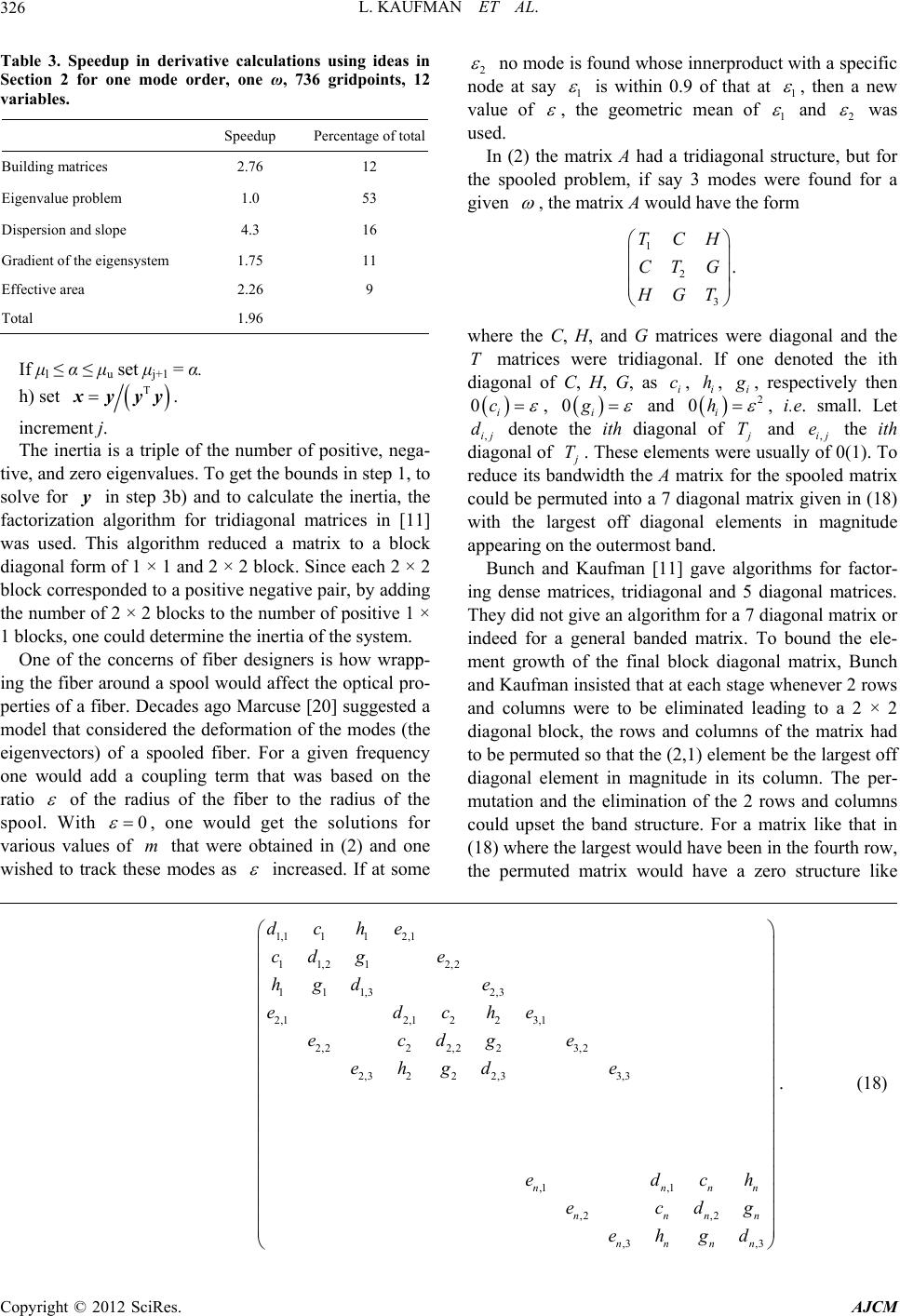
j
ul



.

L. KAUFMAN ET AL. 326
Table 3. Speedup in derivative calculations using ideas in
Section 2 for one mode order, one ω, 736 gridpoints, 12
variables.
Speedup Percentage of total
Building matrices 2.76 12
Eigenvalue problem 1.0 53
Dispersion and slope 4.3 16
Gradient of the eigensystem 1.75 11
Effective area 2.26 9
Total 1.96
2

no mode is found whose innerproduct with a specific
node at say 1

is within 0.9 of that at 1

, then a new
value of

, the geometric mean of 1

and 2

was
used.
In (2) the matrix A had a tridiagonal structure, but for
the spooled problem, if say 3 modes were found for a
given

, the matrix A would have the form
1
2
3
.
TCH
CT G
H
GT





where the C, H, and G matrices were diagonal and the
matrices were tridiagonal. If one denoted the ith
diagonal of C, H, G, as i, ,
T
ci hi
g
, respectively then


i
c0


,


0i g


and

i
h2 0

, i.e. small. Let
,ij denote the ith diagonal of d
j
T and ,ij the ith
diagonal of
e
j
T. These elements were usually of 0(1). To
reduce its bandwidth the A matrix for the spooled matrix
could be permuted into a 7 diagonal matrix given in (18)
with the largest off diagonal elements in magnitude
appearing on the outermost band.
If μl ≤ α ≤ μu set μj+1 = α.
h) set

T
x
yyy
.
increment j.
The inertia is a triple of the number of positive, nega-
tive, and zero eigenvalues. To get the bounds in step 1, to
solve for
y
in step 3b) and to calculate the inertia, the
factorization algorithm for tridiagonal matrices in [11]
was used. This algorithm reduced a matrix to a block
diagonal form of 1 × 1 and 2 × 2 block. Since each 2 × 2
block corresponded to a positive negative pair, by adding
the number of 2 × 2 blocks to the number of positive 1 ×
1 blocks, one could determine the inertia of the system.
Bunch and Kaufman [11] gave algorithms for factor-
ing dense matrices, tridiagonal and 5 diagonal matrices.
They did not give an algorithm for a 7 diagonal matrix or
indeed for a general banded matrix. To bound the ele-
ment growth of the final block diagonal matrix, Bunch
and Kaufman insisted that at each stage whenever 2 rows
and columns were to be eliminated leading to a 2 × 2
diagonal block, the rows and columns of the matrix had
to be permuted so that the (2,1) element be the largest off
diagonal element in magnitude in its column. The per-
mutation and the elimination of the 2 rows and columns
could upset the band structure. For a matrix like that in
(18) where the largest would have been in the fourth row,
the permuted matrix would have a zero structure like
One of the concerns of fiber designers is how wrapp-
ing the fiber around a spool would affect the optical pro-
perties of a fiber. Decades ago Marcuse [20] suggested a
model that considered the deformation of the modes (the
eigenvectors) of a spooled fiber. For a given frequency
one would add a coupling term that was based on the
ratio

of the radius of the fiber to the radius of the
spool. With 0


m
, one would get the solutions for
various values of that were obtained in (2) and one
wished to track these modes as

increased. If at some
1,1 112,1
11,21 2,2
111,32,3
2,12,1 223,1
2,22 2,2 23,2
2,3 222,33,3
,1 ,1
,2 ,2
,3 ,3
nnn
nnn
nnnn
dche
cd ge
hgde
edche
ecdge
ehgd e
edc
ecd
ehgd



















n
n
h
g
. (18)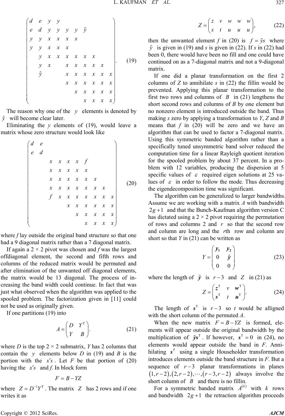

L. KAUFMAN ET AL. 327
.
deyy
edyyyyy
yyxxxx
yyxxx
yxxxxxx
yx xxxxx
yxxxxxx
x
xxxxx
x
xxxx
x
xxx






























(19)
The reason why one of the elements is denoted by y
y
 will become clear later.
Eliminating the y elements of (19), would leave a
matrix whose zero structure would look like
de
ed
xxxxf
xxxxx
xxxxxx
xxxxxxx
f
xxxxxxx
x
xxxxx
x
xxxx
x
xxx

































(20)
where f lay outside the original band structure so that one
had a 9 diagonal matrix rather than a 7 diagonal matrix.
If again a 2 × 2 pivot was chosen and f was the largest
offdiagonal element, the second and fifth rows and
columns of the reduced matrix would be permuted and
after elimination of the unwanted off diagonal elements,
the matrix would be 13 diagonal. The process of in-
creasing the band width could continue. In fact that was
just what observed when the algorithm was applied to the
spooled problem. The factorization given in [11] could
not be used as originally given.
If one partitions (19) into
T
.
DY
AYB



(21)
where D is the top 2 × 2 submatrix, Y has 2 columns that
contain the elements below D in (19) and B is the
portion with the
y
x
s
. Let F be that portion of (20)
having the
x
s
 and f. In block form
F
BYZ
where 1T
Z
DY

. The matrix
Z
has 2 rows and if one
writes it as
,
zvwww
Z
s
tuuu



(22)
then the unwanted element f in (20) is
f
ys where
y
 is given in (19) and s is given in (22). If s in (22) had
been 0, there would have been no fill and one could have
continued on as a 7-diagonal matrix and not a 9-diagonal
matrix.
If one did a planar transformation on the first 2
columns of Z to annihilate s in (22) the fillin would be
prevented. Applying this planar transformation to the
first two rows and columns of in (21) lengthens the
short second rows and columns of B by one element but
no nonzero element is introduced outside the band. Thus
making s zero by applying a transformation to Y, Z and B
means that f in (20) will be zero and we have an
algorithm that can be used to factor a 7-diagonal matrix.
Using this symmetric banded algorithm rather than a
specifically tuned unsymmetric band solver reduced the
computation time for a linear Rayleigh quotient iteration
for the spooled problem by about 37 percent. In a pro-
blem with 12 variables, producing the dispersion at 5
specific values of
B

required eigen solutions at 25 va-
lues of

in order to follow the mode. Thus decreasing
the eigendecomposition time was significant.
The algorithm can be generalized to larger bandwidths.
Assume we are working with a matrix A with bandwidth
21
g

and that the Bunch-Kaufman algorithm version C
has dictated using a 2 × 2 pivot requiring the permutation
of rows and columns 2 and so that the second row
and column are long and the row and column are
short so that Y in (21) can be written as
r
rth
0
00
Y





yy
y

12


(23)
where the length of is and
y
3r
Z
in (21) as
TT
TT
.
v
Zt



zw
su

(24)
The length of is
T
s3r

so t would be alligned
with the short column of the permuted A.
When the new matrix
F
BYZ
T
s
is formed, ele-
ments will appear outside the original bandwidth by the
multiplication of . If however, in (24), no
elements would appear outside the band in F. Anni-
hilating using a single Householder transformation
introduces elements outside the band structure in F. But a
sequence of r
T
ys

3
0
T
s

planar transformations in planes






3, 2rr1,2rr, 2,2,,


B

k
always involve the
short column of and there is no fillin.
For a symmetric banded matrix

A
with rows
and bandwidth
k
21
g

the retraction algorithm proceeds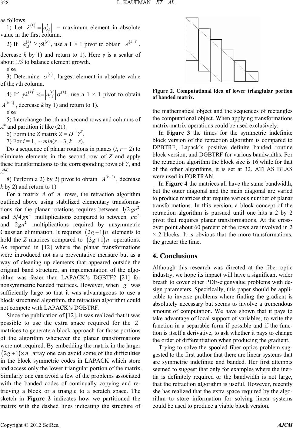

L. KAUFMAN ET AL. 328
as follows
1) Let

,1
kk
r
a   = maximum element in absolute
value in the first column.
2) If
 
1,1
k
ak

 , use a 1 × 1 pivot to obtain

1k
A

,
decrease k by 1) and return to 1). Here γ is a scalar of
about 1/3 to balance element growth.
else
3) Determine

k

, largest element in absolute value
of the rth column.
4) If
 
2
1,1
kk
ak

   , use a 1 × 1 pivot to obtain

1k
A
, decrease k by 1) and return to 1).
else
5) Interchange the rth and second rows and columns of
Ak and partition it like (21).
6) Form the Z matrix Z = D−1YT.
7) For i = 1, ··· min(r − 3, k − r).
Do a sequence of planar rotations in planes (i, r − 2) to
eliminate elements in the second row of Z and apply
these transformations to the corresponding rows of Y, and
A(k)
8) Perform a 2) by 2) pivot to obtain

2k
A
, decrease
k by 2) and return to 1)
For a matrix A of rows, the retraction algorithm
outlined above using stabilized elementary transforma-
tions for the planar rotations requires between
n
2
12
g
n
and 2 54
g
n multiplications compared to between 2
g
n
and 2 2
g
n multiplications required by unsymmetric
Gaussian elimination. It requires

21

g
n

31
elements to
hold the Z matrices compared to

g
n operations.
As reported in [12] where the planar transformations
were introduced not as a preventative measure but as a
way of cleaning up elements that appeared outside the
original band structure, an implementation of the algo-
rithm was faster than LAPACK’s DGBTF2 [21] for
nonsymmetric banded matrices. However, when
g
was
sufficiently large so that it was advantageous to use a
block structured algorithm, the retraction algorithm could
not compete with LAPACK’s DGBTRF.
Since the publication of [12], it was realized that it was
possible to use the extra space required for the
Z
matrices to generate a block approach for those portions
of the algorithm whenever the planar transformations
were not required. By embedding the matrix in the larger

21
g
n array one can avoid some of the difficulties
in the block symmetric codes in LAPACK which store
and access only the lower triangular portion of the matrix.
Similarly one can avoid a few of the problems associated
with the banded codes of continually copying and re-
trieving a block or a triangle to a scratch space. The
sketch in Figure 2 indicates how we partitioned the
matrix with the dashed lines indicating the structure of
Figure 2. Computational idea of lower trianglular portion
of banded matrix.
the mathematical object and the sequences of rectangles
the computational object. When applying transformations
matrix-matrix operations could be used exclusively.
In Figure 3 the times for the symmetric indefinite
block version of the retraction algorithm is compared to
DPBTRF, Lapack’s positive definite banded routine
block version, and DGBTRF for various bandwidths. For
the retraction algorithm the block size is 16 while for that
of the other algorithms, it is set at 32. ATLAS BLAS
were used in FORTRAN.
In Figure 4 the matrices all have the same bandwidth,
but the outer diagonal and the main diagonal are varied
to produce matrices that require various number of planar
transformations. In this version, a block concept of the
retraction algorithm is pursued until one hits a 2 by 2
pivot that requires planar transformations. At the cross-
over point about 60 percent of the rows are involved in 2
× 2 blocks. It is obvious that the more transformations,
the greater the time.
4. Conclusions
Although this research was directed at the fiber optic
industry, we hope its impact will have a significant wider
breath to cover other PDE-eigenvalue problems with de-
sign parameters. Specifically, this paper should be appli-
cable to inverse problems where finding the gradient is
absolutely necessary but seems to involve a tremendous
amount of computation. We have shown that it pays to
take advantage of local support of variables, to write the
function in a separable form if possible and if the func-
tion is itself a derivative, to ask whether it pays to change
the order of differentiation when producing the gradient.
Trying to solve the spooled fiber optics problem sug-
gested to the first author that there are linear systems that
are symmetric indefinite and banded. Her first attempts
seemed to suggest that only for examples where the iner-
tia is definitely required or the bandwidth is not large,
that the retraction algorithm is useful. However, recently
she has realized that the extra space required by the algo-
rithm to store information for solving linear systems
could be used to produce a viable block version.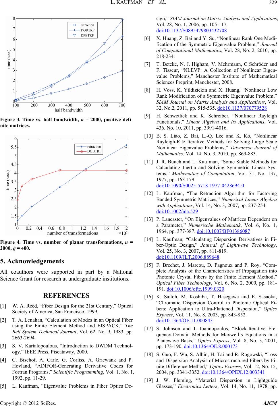

L. KAUFMAN ET AL. 329
Figure 3. Time vs. half bandwidth, n = 2000, positive defi-
nite matrices.
Figure 4. Time vs. number of planar transformations, n =
2000, g = 400.
5. Acknowledgements
All coauthors were supported in part by a National
Science Grant for research at undergraduate institutions.
REFERENCES
[1] W. A. Reed, “Fiber Design for the 21st Century,” Optical
Society of America, San Francisco, 1999.
[2] T. A. Lenahan, “Calculation of Modes in an Optical Fiber
using the Finite Element Method and EISPACK,” The
Bell System Technical Journal, Vol. 62, No. 9, 1983, pp.
2663-2694.
[3] S. V. Kartalopoulous, “Introduction to DWDM Technol-
ogy,” IEEE Press, Piscataway, 2000.
[4] C. Bischof, A. Carle, G. Corliss, A. Griewank and P.
Hovland, “ADIFOR-Generating Derivative Codes for
Fortran Programs,” Scientific Programming, Vol. 1, No. 1,
1992, pp. 11-29.
[5] L. Kaufman, “Eigenvalue Problems in Fiber Optics De-
sign,” SIAM Journal on Matrix Analysis and Applications,
Vol. 28, No. 1, 2006, pp. 105-117.
doi:10.1137/S0895479803432708
[6] X. Huang, Z. Bai and Y. Su, “Nonlinear Rank One Modi-
fication of the Symmetric Eigenvalue Problem,” Journal
of Computational Mathematics, Vol. 28, No. 2, 2010, pp.
218-234.
[7] T. Betcke, N. J. Higham, V. Mehrmann, C Schröder and
F. Tisseur, “NLEVP: A Collection of Nonlinear Eigen-
value Problems,” Manchester Institute of Mathematical
Sciences Preprint, Manchester, 2008.
[8] H. Voss, K. Yildiztekin and X. Huang, “Nonlinear Low
Rank Modification of a Symmetric Eigenvalue Problem,”
SIAM Journal on Matrix Analysis and Applications, Vol.
32, No.2, 2011, pp. 515-535. doi:10.1137/070779528
[9] H. Schwetlick and K. Schreiber, “Nonlinear Rayleigh
Functionals,” Linear Algebra and its Applications, Vol.
436, No. 10, 2011, pp. 3991-4016.
[10] B. S. Liao, Z. Bai, L.-Q. Lee and K. Ko, “Nonlinear
Rayleigh-Ritz Iterative Methods for Solving Large Scale
Nonlinear Eigenvalue Problems,” Taiwanese Journal of
Mathematics, Vol. 14, No. 3, 2010, pp. 869-883.
[11] J. R. Bunch and L. Kaufman, “Some Stable Methods for
Calculating Inertia and Solving Symmetric Linear Sys-
tems,” Mathematics of Computation, Vol. 31, No. 137,
1977, pp. 163-179.
doi:10.1090/S0025-5718-1977-0428694-0
[12] L. Kaufman, “The Retraction Algorithm for Factoring
Banded Symmetric Matrices,” Numerical Linear Algebra
with Applications, Vol. 14, No. 3, 2007, pp. 237-254.
doi:10.1002/nla.529
[13] P. Lancaster, “On Eigenvalues of Matrices Dependent on
a Parameter,” Numerische Mathematik, Vol. 6, No. 1,
1964, pp. 377-387. doi:10.1007/BF01386087
[14] L. Kaufman, “Calculating Dispersion Derivatives in Fi-
ber-Optic Design,” Journal of Lightwave Technology,
Vol. 25, No. 3, 2007, pp. 811-819.
doi:10.1109/JLT.2006.889648
[15] F. Brechet, J. Marcou, D. Pagnoux and P. Roy, “Com-
plete Analysis of the Characteristics of Propagation into
Photonic Crystal Fibers by the Finite Element Method,”
Optical Fiber Technology, Vol. 6, No. 2, 2000, pp. 181-
191. doi:10.1006/ofte.1999.0320
[16] K. Saitoh, M. Koshiba, T. Hasegawa and E. Sasaoka,
“Chromatic Dispersion Control in Photonic Optical Fi-
bers: Application to Ultra-Flattened Dispersion,” Optics
Express, Vol. 11, No. 8, 2003, pp. 843-852.
doi:10.1364/OE.11.000843
[17] S. Johnson and J. Joannopoulos, “Block-Iterative Fre-
quency-Domain Methods for Maxwell’s Equations in a
Planewave Basis,” Optics Express, Vol. 8, No. 3, 2001,
pp. 173-190. doi:10.1364/OE.8.000173
[18] S. Guo, F. Wu, S. Albin, H. Tai and R. Rogowski, “Loss
and Dispersion Analysis of Microstructured Fibers by Fi-
nite Difference Method,” Optics Express, Vol. 12, No. 15,
2004, pp. 3341-3352. doi:10.1364/OPEX.12.003341
[19] J. W. Fleming, “Material Dispersion in Lightguide
Glasses,” Electronics Letters, Vol. 14, No. 11, 1978, pp.

L. KAUFMAN ET AL. 330
326-328. doi:10.1049/el:19780222
[20] D. Marcuse, “Field Deformation and Loss Caused by
Curvature of Optical Fibers,” Journal of the Optical Soci-
ety America, Vol. 66, No. 4, 1972, pp. 311-320.
doi:10.1364/JOSA.66.000311
[21] E. Anderson, Z. Bai, C. Bischof, J. Demmel, J. Dongarra,
J. Du Croz, A. Greenbaum, S. Hammarling, A.
McKenney, S. Ostrouchov and D. Sorensen, “LAPACK
Users’ Guide,” 2nd Edition, Society for Industrial and
Applied Mathematics, Philadelphia, 1995.