Journal of Environmental Protection, 2010, 1, 242-250
doi:10.4236/jep.2010.13029 Published Online September 2010 (http://www.SciRP.org/journal/jep)
Remote Mapping of Thermodynamic Index of
Ecosystem Health Disturbance
Victor I. Gornyy, Sergei G. Kritsuk, Iscander Sh. Latypov
Saint-Petersburg Scientific Research Center for Ecological Safety, Russian Academy of Sciences, Saint-Petersburg, Russia.
Received May 4th, 2010; revised June 15th, 2010; accepted June 18th, 2010.
ABSTRACT
The study of the ecological system (ES) reaction to anthropogenous loading (AL) has been aimed at developing the re-
mote sensing method for quantitative mapping of AL on ES. The analysis of the problem has shown that the main ap-
proach for its solution is to assess the amount of entropy induced in ES by AL. The general formalism has been dis-
cussed and the thermodynamic index of ES health disturbance (TIEHD- T
I
) has been deduced from the conservation
law as a portion of solar exergy spent by ES on the parrying entropy formed in ES due to AL with respect to the total
amount of exergy of solar irradiations absorbed by ES. The technique of remote mapping of TIEHD has been developed.
The maps of TIEHD and the normalized differential vegetation index (NDVI)-V
I
have been compiled on the basis of
NOAA and EOS satellite data. The qualitative and quantitative analysis exhibited the best sensitivity of TIEHD to AL on
ES in respect to NDVI.
Keywords: Ecosystem, Thermodynamics, Anthropogenous Loading, Satellite, Index
1. Introduction
Quantitative estimation of ES health affected by AL is
one of the most challenging problems of environmental
state monitoring. In terms of economy remote sensing
technology is the most convenient for carrying out opera-
tional monitoring of ES reaction to AL.
There have been numerous attempts to create tech-
niques for assessing AL on ES [1,2]. These techniques
are mainly based on the method of induction (from the
particular to the general) using numerous quantitative
indicators, e.g., indices, describing [1]:
1) the biogeochemical substance and energy cycles;
2) the actual or potential productivity of the ES;
3) the biodiversity of the ecosystems (Species Rich-
ness, ES Scarcity, ES Vulnerability);
4) the cultural value of the affected sites;
5) the migration and dispersal of species composition.
W. M. Achten, E. Mathijas, B. Muys [3] based their
ES health criteria system on two factors: impact on the
ES Structural Quality (Soil fertility, Biomass production,
Species diversity) and ES Functional Quality (Soil struc-
ture, Vegetation structure, On-site water balance). The
authors suggested 22 indicators of AL on ES and the
principle of indicators generalization: “…the impact in-
dicator scores as the summation of the relative impacts
of the different land use activities” [3].
Our analysis of the above mentioned factors leads to
the conclusion that this methodology of assessment of
AL on ES cannot be implemented in a real operational
mode due to its high complexity and for economic rea-
sons.
There are two different approaches to the solution of
scientific problems: microscopic and macroscopic. Sta-
tistical thermodynamics, for example, uses the micro-
scopic approach, first, to derive parameters of kinematics
and dynamics for each particle of ideal gas, then, to de-
scribe the type of chaos, further, to take into account the
type of interactions between particles and, finally, to ob-
tain some integrated parameters of the investigated object,
e.g. a spatial temperature distribution in the ideal gas.
However, the same result (temperature distribution in a
solid body) can be more easily obtained using the mac-
roscopic approach. In this case some general parameters
of the heat transfer in a solid body (a thermal conductiv-
ity, a thermal capacity and a density) are to be measured,
followed by a boundary value problem solution of heat
transfer using Fourier differential equation. This ap-
proach needs much less effort to obtain the same result
than the first case.

Remote Mapping of Thermodynamic Index of Ecosystem Health Disturbance 243
The results in [1,3] have been obtained using the mi-
croscopic approach (collecting a large number of differ-
ent indicators for each ES element and compiling a gen-
eralized index). Therefore it was found reasonable to
make an attempt to create a generalized index of AL on
ES using the macroscopic approach. These attempts were
made in the framework of the ES thermodynamic theory
[4-9].
The main idea of the thermodynamic approach of ES
health assessment is to reveal changes of generalized ES
thermodynamic parameters caused by AL. Especially
noteworthy is the paper concerned mainly with philoso-
phical problems of the thermodynamics of biological
organisms by E. D. Schnider and J. J. Kay [5] who for-
mulated nine principles of thermodynamic state of ES. T.
Wagendorp et al. reduced these principles to two basic
ones (these methods of assessment of ES reaction to AL
are discussed in [9]). Their technique includes a descrip-
tion of the structural state of the ES (goal function:
maximum exergy1 storage) and the function caused by
the low entropy system (goal function: maximum exergy
dissipation). According to T. Wagendorp et al. only two
indices can be used for remote mapping: thermal re-
sponse number (ITRN) and solar exergy dissipation (ISED),
put forward by J. C. Luvall and H. R. Holbo [7] as:
2
1
[() /]
TRN ns
I
RT


 
 (1)
where n
R is the net incoming radiation; 21 ()

 
is the time interval between two successive remote sens-
ing surveys;
s
T is the change of surface temperature
s
T between moments of time 1

and 2

.
*
/
SED n
I
RK (2)
where *
K
is the net shortwave radiation.
ISED represents the fraction of the net radiation that is
dissipated into a heat – the type of energy with a lower
level of exergy. It reflects an exergy degradation and
storage in a system [5]. J. C. Luvall and H. R. Holbo
mapped TRN
I
and SED
I
applying airborne multispectral
survey with the help of a Thermal Infrared Multichannel
Scanner (TIMS) [7].
The analysis of these two indices has shown the fol-
lowing deficiencies:
1) these two indices have not been deduced from the
basic physical laws, but were suggested empirically;
2) TRN
I
is the palliative of the thermal inertia (TI)
(see [10-14] for details).
The TI reflects the resistance of the surface to the pe-
riodic process of heating and cooling. Being a bulk prop-
erty, TI does not depend on the time of observation and
weather conditions. TRN
I
, being just a characteristics,
depends on different natural factors. That is why it is
impossible to quantitatively compare TRN
I
obtained on
different dates, even for the same ES.
The best results in the macroscopic approach have
been achieved by S. E. Jorgensen and Yu. Svirezhev in
their monograph on the general thermodynamic theory of
ES [4]. The authors demonstrated that the general ther-
modynamic measure of AL on ES is the additional pro-
duction of entropy


taking place in the time interval


[4]:
[()( )]
ˆˆ
[]/;
oo
fch o
SS
WW PPT


 


 
 (3)
where: S is the entropy of ES; ˆ
f
W is the total energy
loading on ES; ˆch
W is the total chemical loading on ES;
P is the gross primary production measured in mass of
carbon per unit area per year: (g Carbon/m2/yr). The
gross primary production is the speed at which an ES
stores a given amount of chemical energy as a biomass in
a given time interval. P is the mean gross primary
production averaged over the

 time of AL; o P is the
initial gross primary production of ES for the moment of
time: o

, when AL was applied; T is the absolute
temperature of ES (assumed constant during all time in-
terval


); o



 ;

is the ongoing moment of
time.
The analysis of Equation (3) shows that remote meas-
urements of 0
ˆ,,,
f
WPPT are possible to make. How-
ever, to determine remotely, the chemical loading (ˆch
W),
is very difficult due to a large number of uncertainties
making it impossible to use Equation (3) directly. Thus,
the main target of this paper is to develop TIEHD that
can be mapped remotely, based on general thermody-
namic considerations.
The outline of the paper is as follows: Section 2 pre-
sents our formalism and derives a general formula for
TIEHD. Section 3 deals with materials and methods.
Section 4 shows the results for the industrial Urals region,
one of the most industrialized and polluted areas of Rus-
sia. Discussion and conclusions are presented in Section
5 and Section 6.
2. General Formalism
Following the major works concerned with the thermo-
dynamic theory of ES [4,5,9] we suggest that ES and the
environment is a supersystem and the environment is
much larger than ES. According to Equation (3) AL
1Ex-exergy is the maximum work, which ES can perform during the
pr
ocess of reaching the state of equilibrium with the environment [4].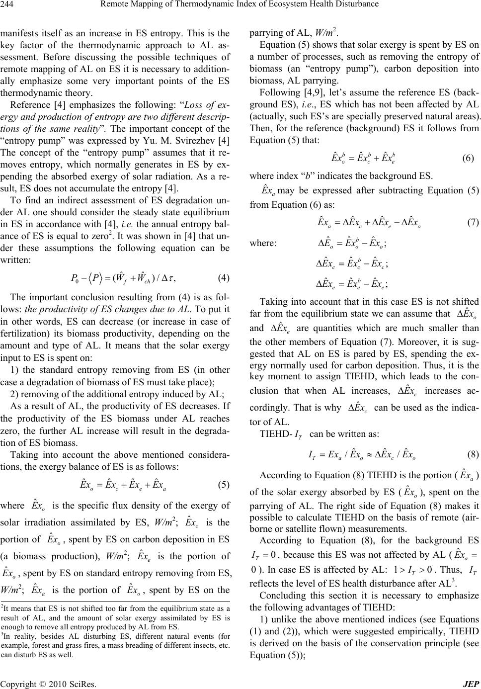

Remote Mapping of Thermodynamic Index of Ecosystem Health Disturbance 244
manifests itself as an increase in ES entropy. This is the
key factor of the thermodynamic approach to AL as-
sessment. Before discussing the possible techniques of
remote mapping of AL on ES it is necessary to addition-
ally emphasize some very important points of the ES
thermodynamic theory.
Reference [4] emphasizes the following: “Loss of ex-
ergy and production of entropy are two different descrip-
tions of the same reality”. The important concept of the
“entropy pump” was expressed by Yu. M. Svirezhev [4]
The concept of the “entropy pump” assumes that it re-
moves entropy, which normally generates in ES by ex-
pending the absorbed exergy of solar radiation. As a re-
sult, ES does not accumulate the entropy [4].
To find an indirect assessment of ES degradation un-
der AL one should consider the steady state equilibrium
in ES in accordance with [4], i.e. the annual entropy bal-
ance of ES is equal to zero2. It was shown in [4] that un-
der these assumptions the following equation can be
written:
0ˆˆ
()/,
fch
PP WW

  (4)
The important conclusion resulting from (4) is as fol-
lows: the productivity of ES changes due to AL. To put it
in other words, ES can decrease (or increase in case of
fertilization) its biomass productivity, depending on the
amount and type of AL. It means that the solar exergy
input to ES is spent on:
1) the standard entropy removing from ES (in other
case a degradation of biomass of ES must take place);
2) removing of the additional entropy induced by AL;
As a result of AL, the productivity of ES decreases. If
the productivity of the ES biomass under AL reaches
zero, the further AL increase will result in the degrada-
tion of ES biomass.
Taking into account the above mentioned considera-
tions, the exergy balance of ES is as follows:
ˆ ˆˆˆ
o cea
ExEx Ex Ex (5)
where ˆo Ex is the specific flux density of the exergy of
solar irradiation assimilated by ES, W/m2; ˆc
Ex is the
portion of ˆo
Ex , spent by ES on carbon deposition in ES
(a biomass production), W/m2; ˆe Ex is the portion of
ˆo
Ex , spent by ES on standard entropy removing from ES,
W/m2; ˆa
Ex is the portion of ˆo Ex , spent by ES on the
parrying of AL, W/m2.
Equation (5) shows that solar exergy is spent by ES on
a number of processes, such as removing the entropy of
biomass (an “entropy pump”), carbon deposition into
biomass, AL parrying.
Following [4,9], let’s assume the reference ES (back-
ground ES), i.e., ES which has not been affected by AL
(actually, such ES’s are specially preserved natural areas).
Then, for the reference (background) ES it follows from
Equation (5) that:
ˆˆˆ
bbb
oce
ExEx Ex (6)
where index “b” indicates the background ES.
ˆa
Ex may be expressed after subtracting Equation (5)
from Equation (6) as:
ˆˆˆˆ
aceo
ExEx Ex Ex  (7)
where: ˆˆ ˆ ;
b
ooo
EExEx 
ˆˆˆ
;
b
ccc
ExExEx 
ˆˆˆ
;
b
eee
ExEx Ex 
Taking into account that in this case ES is not shifted
far from the equilibrium state we can assume that ˆo Ex

and ˆe
Ex

are quantities which are much smaller than
the other members of Equation (7). Moreover, it is sug-
gested that AL on ES is pared by ES, spending the ex-
ergy normally used for carbon deposition. Thus, it is the
key moment to assign TIEHD, which leads to the con-
clusion that when AL increases, ˆc
Ex increases ac-
cordingly. That is why ˆc
Ex can be used as the indica-
tor of AL.
TIEHD- T
I
can be written as:
ˆˆˆ
//
Tao co
I
ExExEx Ex (8)
According to Equation (8) TIEHD is the portion (ˆa Ex )
of the solar exergy absorbed by ES (ˆo Ex ), spent on the
parrying of AL. The right side of Equation (8) makes it
possible to calculate TIEHD on the basis of remote (air-
borne or satellite flown) measurements.
According to Equation (8), for the background ES
0
T
I

, because this ES was not affected by AL (ˆa Ex

0). In case ES is affected by AL: 10
T
I. Thus, T
I
reflects the level of ES health disturbance after AL3.
Concluding this section it is necessary to emphasize
the following advantages of TIEHD:
1) unlike the above mentioned indices (see Equations
(1) and (2)), which were suggested empirically, TIEHD
is derived on the basis of the conservation principle (see
Equation (5));
2It means that ES is not shifted too far from the equilibrium state as a
result of AL, and the amount of solar exergy assimilated by ES is
enough to remove all entropy produced by AL from ES.
3In reality, besides AL disturbing ES, different natural events (fo
r
example, forest and grass fires, a mass breading of different insects, etc.
can disturb ES as well.

Remote Mapping of Thermodynamic Index of Ecosystem Health Disturbance 245
2) it can be suggested that TIEHD is more sensitive to
AL than remotely measured vegetation indices, as
TIEHD reflects the changes in the physiological process
of vegetation (transpiration and photosynthesis).
Therefore, the remote mapping of the rate of carbon
deposition and ˆo
Ex provides the possibility to compile
a map of TIEHD.
3. Materials and Methods
3.1. Test Site
The south-eastern Urals region of Russia has been cho-
sen as the test site (the Urals Test Site (UTS)) for TIEHD
remote mapping (Figure 1).
The climate of UTS is continental with long cold win-
ters and relatively short and warm summers [15]. There
are three biomes within the UTS territory: boreal forest
(UTS Western part), South of West Siberian forest steppe,
and steppe (UTS Eastern part) [15].
There are two major geomorphologic forms within the
UTS territory: Trans-Urals peneplain (UTS Western part)
and West Siberian lowland (Eastern part).
The UTS territory lies in one of Russia's oldest indus-
trial regions with a large number of metallurgical, met-
alworking, engineering, and chemical enterprises. The
biggest industrial centers are the cities of Chelyabinsk,
Karabash, Kopeisk, Miass, Zlatoust (see Figure 1).
Figure 1. The schematic map of the UTS.
The main requirements for TIEHD remote mapping
technique verification were the following: the total range
of AL on ES has to be varied from maximum to mini-
mum; the test site ES has to be homogeneous enough and
the AL source has to be unique.
The city of Karabash in Chelyabinsk Oblast’ is the one
of such places within UTS (Figure 1).
The city of Karabash is located in a mountainous taiga
area. The main species of the forests are spruce, silver fir
and an admixture of pines, mountain ashes and junipers.
The soil is mountainous podzol. The main wind direction
is latitudinal. The city is situated in the depression of the
surface relief.
The copper smelting plant was built in the city of
Karabash early in the 19th century. Besides, the smelting
of complex sulfide ores started at the beginning of the
20th century. As a result, the surrounding ES was sig-
nificantly affected by this enterprise at the end of the
20th century. For example, during the peak of the Kara-
bash enterprise production (till 1989) about 160-180 th-
ousand tons of pollutants in the form of smoke, dust and
gases were thrown out into the atmosphere annually.
About 90% of it was sulfur dioxide, the others being lead,
copper, zinc, arsenic, as well as carbon oxide, nitrogen
dioxide, etc. 12 million tons of harmful substances have
been thrown out into the atmosphere during all the time
of the industrial complex activity. As a result, ES around
the city of Karabash has been affected by the hard AL
during a long time period. This is illustrated in the map
of NDVI-V
I
(see Figure 5). The broad area of dead
vegetation can be observed inside and around the city of
Karabash.
3.2. Data
Terra(MODIS) satellite data were used to calculate ˆo Ex
(Equation (9), Table 1).
3.3. ˆo
E
x Mapping
The ˆo Ex can be measured remotely using the technique
described by S. Yorgensen and Yu. Svirezhev [4]:
ˆ() [()/()]
[1(ln1) / (1)];
outout in
o
ExQLn QQdR
RKu

 




 (9)
where out
Q, in Q are the outgoing and the ingoing spe-
cific densities of solar irradiation fluxes respectively,
W/m2;

is the frequency of light spectrum;

is the
total measured spectral interval; 0
1
log( /)
n
iii
i
K
ppp


is Kullback’s measure; 0
ii
p,p probabilities before and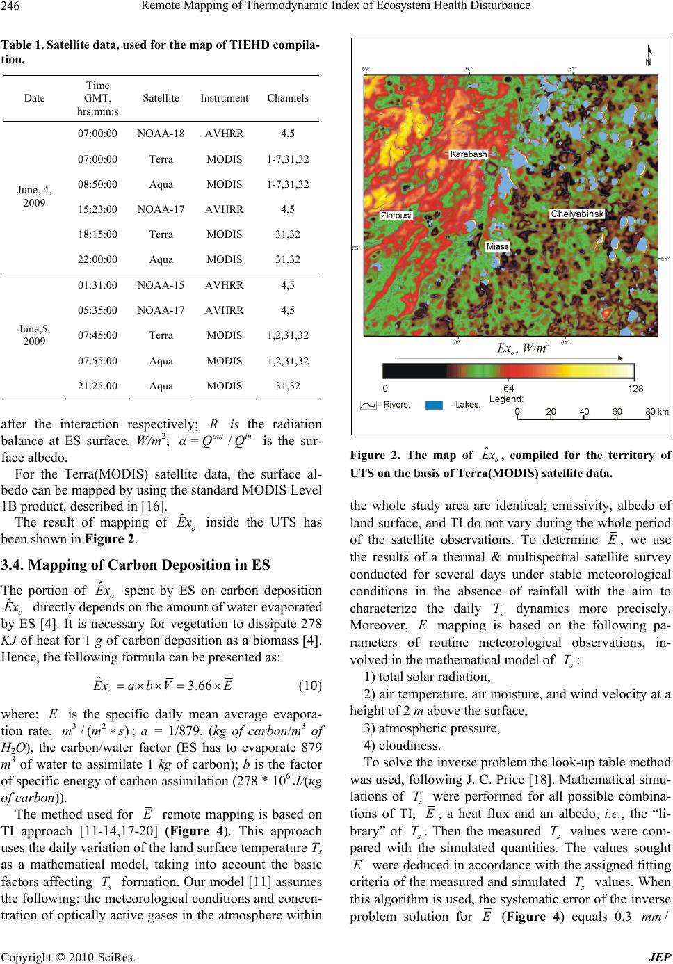

Remote Mapping of Thermodynamic Index of Ecosystem Health Disturbance 246
Table 1. Satellite data, used for the map of TIEHD compila-
tion.
Date
Time
GMT,
hrs:min:s
Satellite Instrument Channels
07:00:00 NOAA-18 AVHRR 4,5
07:00:00 Terra MODIS 1-7,31,32
08:50:00 Aqua MODIS 1-7,31,32
15:23:00 NOAA-17 AVHRR 4,5
18:15:00 Terra MODIS 31,32
June, 4,
2009
22:00:00 Aqua MODIS 31,32
01:31:00 NOAA-15 AVHRR 4,5
05:35:00 NOAA-17 AVHRR 4,5
07:45:00 Terra MODIS 1,2,31,32
07:55:00 Aqua MODIS 1,2,31,32
June,5,
2009
21:25:00 Aqua MODIS 31,32
after the interaction respectively; R is the radiation
balance at ES surface, W/m2; /
out in
α=QQ is the sur-
face albedo.
For the Terra(MODIS) satellite data, the surface al-
bedo can be mapped by using the standard MODIS Level
1B product, described in [16].
The result of mapping of ˆo
Ex inside the UTS has
been shown in Figure 2.
3.4. Mapping of Carbon Deposition in ES
The portion of ˆo Ex spent by ES on carbon deposition
ˆc
Ex directly depends on the amount of water evaporated
by ES [4]. It is necessary for vegetation to dissipate 278
KJ of heat for 1 g of carbon deposition as a biomass [4].
Hence, the following formula can be presented as:
ˆ3.66
c
Exab VE  (10)
where: E is the specific daily mean average evapora-
tion rate, 32 /( )mms; a = 1/879, (kg of carbon/m3 of
H2O), the carbon/water factor (ES has to evaporate 879
m3 of water to assimilate 1 kg of carbon); b is the factor
of specific energy of carbon assimilation (278 * 106 J/(кg
of carbon)).
The method used for E remote mapping is based on
TI approach [11-14,17-20] (Figure 4). This approach
uses the daily variation of the land surface temperature Ts
as a mathematical model, taking into account the basic
factors affecting
s
T formation. Our model [11] assumes
the following: the meteorological conditions and concen-
tration of optically active gases in the atmosphere within
Figure 2. The map of ˆo
Ex , compiled for the territory of
UTS on the basis of Terra(MODIS) satellite data.
the whole study area are identical; emissivity, albedo of
land surface, and TI do not vary during the whole period
of the satellite observations. To determine E, we use
the results of a thermal & multispectral satellite survey
conducted for several days under stable meteorological
conditions in the absence of rainfall with the aim to
characterize the daily
s
T dynamics more precisely.
Moreover, E mapping is based on the following pa-
rameters of routine meteorological observations, in-
volved in the mathematical model of
s
T:
1) total solar radiation,
2) air temperature, air moisture, and wind velocity at a
height of 2 m above the surface,
3) atmospheric pressure,
4) cloudiness.
To solve the inverse problem the look-up table method
was used, following J. C. Price [18]. Mathematical simu-
lations of
s
T were performed for all possible combina-
tions of TI, E, a heat flux and an albedo, i.e., the “li-
brary” of
s
T. Then the measured
s
T values were com-
pared with the simulated quantities. The values sought
E were deduced in accordance with the assigned fitting
criteria of the measured and simulated
s
T values. When
this algorithm is used, the systematic error of the inverse
problem solution for E (Figure 4) equals 0.3 /mm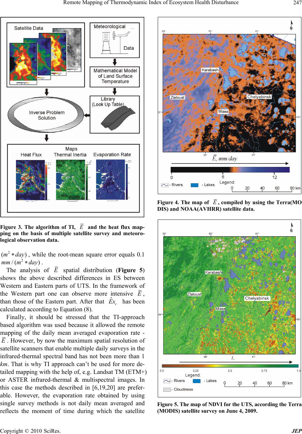

Remote Mapping of Thermodynamic Index of Ecosystem Health Disturbance 247
Figure 3. The algorithm of TI, E and the heat flux map-
ping on the basis of multiple satellite survey and meteoro-
logical observation data.
2
()mday, while the root-mean square error equals 0.1
2
/( )mm mday.
The analysis of E spatial distribution (Figure 5)
shows the above described differences in ES between
Western and Eastern parts of UTS. In the framework of
the Western part one can observe more intensive E,
than those of the Eastern part. After that ˆc
Ex has been
calculated according to Equation (8).
Finally, it should be stressed that the TI-approach
based algorithm was used because it allowed the remote
mapping of the daily mean averaged evaporation rate -
E. However, by now the maximum spatial resolution of
satellite scanners that enable multiple daily surveys in the
infrared-thermal spectral band has not been more than 1
km. That is why TI approach can’t be used for more de-
tailed mapping with the help of, e.g. Landsat TM (ETM+)
or ASTER infrared-thermal & multispectral images. In
this case the methods described in [6,19,20] are prefer-
able. However, the evaporation rate obtained by using
single survey methods is not daily mean averaged and
reflects the moment of time during which the satellite
Figure 4. The map of E, compiled by using the Terra(MO
DIS) and NOAA(AVHRR) satellite data.
Figure 5. The map of NDVI for the UTS, according the Terra
(MODIS) satellite survey on June 4, 2009.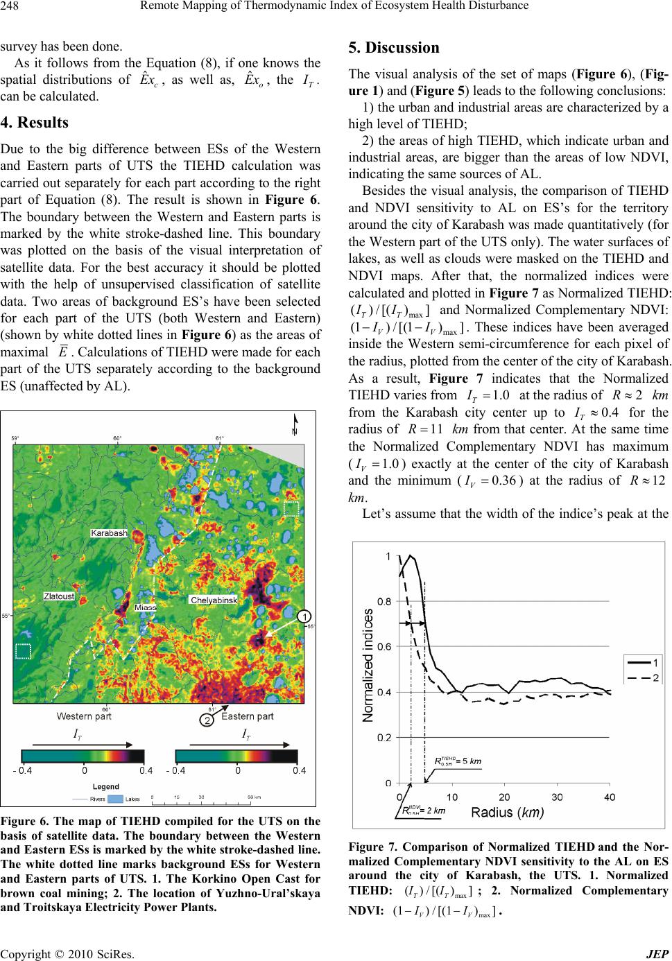

Remote Mapping of Thermodynamic Index of Ecosystem Health Disturbance 248
survey has been done.
As it follows from the Equation (8), if one knows the
spatial distributions of ˆc Ex , as well as, ˆo Ex , the T
I
.
can be calculated.
4. Results
Due to the big difference between ESs of the Western
and Eastern parts of UTS the TIEHD calculation was
carried out separately for each part according to the right
part of Equation (8). The result is shown in Figure 6.
The boundary between the Western and Eastern parts is
marked by the white stroke-dashed line. This boundary
was plotted on the basis of the visual interpretation of
satellite data. For the best accuracy it should be plotted
with the help of unsupervised classification of satellite
data. Two areas of background ES’s have been selected
for each part of the UTS (both Western and Eastern)
(shown by white dotted lines in Figure 6) as the areas of
maximal E. Calculations of TIEHD were made for each
part of the UTS separately according to the background
ES (unaffected by AL).
Figure 6. The map of TIEHD compiled for the UTS on the
basis of satellite data. The boundary between the Western
and Eastern ESs is marked by the white stroke-dashed line.
The white dotted line marks background ESs for Western
and Eastern parts of UTS. 1. The Korkino Open Cast for
brown coal mining; 2. The location of Yuzhno-Ural’skaya
and Troitskaya El ec tricity Pow er Pl ants.
5. Discussion
The visual analysis of the set of maps (Figure 6), (Fig-
ure 1) and (Figure 5) leads to the following conclusions:
1) the urban and industrial areas are characterized by a
high level of TIEHD;
2) the areas of high TIEHD, which indicate urban and
industrial areas, are bigger than the areas of low NDVI,
indicating the same sources of AL.
Besides the visual analysis, the comparison of TIEHD
and NDVI sensitivity to AL on ES’s for the territory
around the city of Karabash was made quantitatively (for
the Western part of the UTS only). The water surfaces of
lakes, as well as clouds were masked on the TIEHD and
NDVI maps. After that, the normalized indices were
calculated and plotted in Figure 7 as Normalized TIEHD:
max
()/[() ]
TT
II and Normalized Complementary NDVI:
max
(1)/ [(1)]
VV
II

. These indices have been averaged
inside the Western semi-circumference for each pixel of
the radius, plotted from the center of the city of Karabash.
As a result, Figure 7 indicates that the Normalized
TIEHD varies from 1.0
T
I

at the radius of 2R

km
from the Karabash city center up to 0.4
T
I for the
radius of 11R

km from that center. At the same time
the Normalized Complementary NDVI has maximum
(1.0
V
I

) exactly at the center of the city of Karabash
and the minimum (0.36
V
I

) at the radius of 12R

km.
Let’s assume that the width of the indice’s peak at the
Figure 7. Comparison of Normalized TIEHD and the Nor-
malized Complementary NDVI sensitivity to the AL on ES
around the city of Karabash, the UTS. 1. Normalized
TIEHD: max ()/[() ]
TT
II ; 2. Normalized Complementary
NDVI: max
(1 )/[(1 )]
VV
II
.

Remote Mapping of Thermodynamic Index of Ecosystem Health Disturbance 249
half of the peak’s height (0.5 2
H
R) indicates the sensitivity
of indices to AL. In this case, for the city of Karabash,
according the Normalized TIEHD the 0.5 210
TIEHD
R

km
(Figure 7), while for the Normalized Complementary
NDVI such width 0.5 24
NDVI
H
R km (Figure 7). This leads
to the conclusion that the sensitivity of TIEHD to AL is
2.5 times better, compared to NDVI.
The highest sensitivity of TIEHD to Al on ES can be
explained by the following considerations. TIEHD is
calculated using such characteristics of vegetation
physiological processes as photosynthesis activity and
quality, as well as water transpiration by leaves. How-
ever, the vegetation index reflects the presence of chlo-
rophyll in ES. That is why, it can be suggested that the
vegetation index records the dramatic stage of vegetation
degradation, when the vegetation has lost chlorophyll
(resulting from forest cuttings, forest and steppe fires or
vegetation death after acid industrial precipitations, as in
the case of the city of Karabash, etc.).
The comparison between TIEHD inside the Western
part of UTS (Figure 6) and TIEHD inside the Eastern
part of UTS shows a big difference, with the Eastern part
having the highest TIEHD. It can be explained by the
landscape difference of these two parts, as well as by
different anthropogenic activity. As can be seen in Fig-
ure 2, the Western part of the UTS is covered by forest,
while the Eastern part is mainly covered by cultivated
fields. The map of TIEHD was compiled for the begin-
ning of summer. For the agriculture & climatic zone of
UTS it is the time with no vegetation on the surface of
fallow fields. As a result, there are areas of the bare soil
here, whose evaporation rate is much lower than that of
the forested area. Thus, TIEHD of the cultivated area for
the beginning of June is much bigger than TIEHD of the
forested area which is not affected by AL.
The big urban and industrial area around the city of
Chelyabinsk is characterized by high TIEHD, resulting
from very big AL on ES. Two more areas of high TIEHD
were investigated additionally. For example, the area of
high TIEHD, situated to the south of the city of Chely-
abinsk (1 in Figure 6) indicates the giant Korkino Open
Cast. Its depth reaches 500 m. The Open Cast supplies
Yuzhno-Ural’skaya and Troitskaya Electric Power Plants
with brown coal. The total power of the Electric Power
Plants is ~ 3000 MW. One of the possible reasons for a
very big area of high TIEHD at the Southern border of
UTS (2 in Figure 6) is the pollution of ES resulting from
the smoke of these Electric Power Plants.
Unlike this situation, water basins (lakes, water ponds,
etc) are surrounded by the zones of very low TIEHD
(Figure 6), as, according to Russia’s legislation the
zones surrounding water basins are territories specially
protected from AL. It is one of the explanations of the
above mentioned phenomenon.
6. Conclusions
To summarize, the major regularities of thermodynamic
reply of ES on AL have been presented and discussed.
Based on the conservation law of exergy fluxes inside ES,
it has been shown that after some simple assumptions
TIEHD can be represented as a portion of solar exergy
spent by ES on the parrying entropy formed in ES due to
AL with respect to the total amount of exergy of solar
irradiations absorbed by ES. It has also been shown that
TIEHD may be mapped on the basis of remote (airborne
or satellite flown) measurements made in the visible,
nearest infrared and infrared-thermal spectral bands by
optic & electronic scanners.
We have chosen the Southern-Eastern Ural region of
Russia as the Test Site and compiled the map of TIEHD
by using NOAA and EOS satellite data. The preliminary
analysis exhibits a better sensitivity of TIEHD to AL on
ES than the NDVI.
It can be concluded that the macroscopic approach (it
was used for the TIEHD compilation) is simpler and less
expensive for the satellite monitoring of AL on ES than
the microscopic approach based on big a number of dif-
ferent indices and their generalization.
The further directions extending our research results
include, in particular, the investigation of TIEHD sea-
sonal dynamic and the detailed ground truth of TIEHD
maps.
7. Acknowledgements
This publication is an output from the research project
Remote sensing methods development for a quantitative
estimation of ES reply on AL No 01.2.007.08 731 funded
by the Russian Academy of Sciences. We thank the
anonymous referee for the constructive criticism and
comments.
REFERENCES
[1] B. P. Weidema, “Physical Impacts of Land Use in Prod-
uct Life Cycle Assessment,” 2001. http://www.lca-net.
com/publications/older/
[2] S. E. Jorgensen, R. Costanza, F. L. Xu, (Eds.) “Handbook
of Ecological Indicators for Assesment of Ecosystem
Health,” Taylor & Frances, 2005.
[3] W. M. J. Achten, E. Mathijs and B. Muys, “Proposing a
Life Cycle Land Use Impact Calculation Methodology,”
Proceedings of 6th International Conference on LCA in
the Agri-Food Sector, Zurich, 12-14 November 2008.
[4] J. S. Jorgensen and Yu. M. Svirezhev, “Towards a Ther-
modynamic Theory for Ecological Systems,” Elsever,
Oxford, 2004.

Remote Mapping of Thermodynamic Index of Ecosystem Health Disturbance 250
[5] E. D. Schnider and J. J. Kay, “Life as a Manifestation of
the Second Law of Thermodynamics,” Mathematical and
Computer Modelling, Vol. 19, No. 6-8, 1994, pp. 25-48.
[6] S. М. Moran, “Chapter 8. Thermal Infrared Measure-
ments as Indicator of Plant Ecosystem Health,” In: D. A.
Quatochi and J. C. Luvall, Eds., Thermal Remote Sensing
in Land Surface Processes, Tailor and Frances, London,
2004, pp. 257-282.
[7] J. C. Luvall and H. R.Holbo, “Measurements of Short
Term Thermal Response of Coniferous Forest Canopies
Using Thermal Scanner Data,” Remote Sensing of Envi-
ronment, Vol. 27, No. 1, 1989, pp. 1-10.
[8] R. D. Jackson, “The Crop Water Stress Index: A Second
Look,” Proceedings of International Conference on Measur-
ment of Soil and Plant Water Stress, Utah State Univer-
sity, July 1987, pp. 87-92.
[9] T. Wagendorp, H. Gulinck, P. Coppin and B. Muys,
“Land Use Impact Evaluation in Life Cycle Assessment
Based on Ecosystem Thermodynamics,” Energy, Vol. 31,
No. 1, 2006, pp. 112-125.
[10] K. Watson, L. C. Rowan and T. V. Offield, “Application
of Thermal Modelling in Geologic Interpretation of IR
Images,” Proceedings of 7th International Symposium on
Remote Sensing of Environment, Ann Arbor, Michigan,
1971, pp. 2017-2041.
[11] V. I. Gornyy, B. V. Shilin and G. I. Yasinskii, “Teplo-
vaya aerokosmocheskaya s’emka (Thermal Airborne and
Satellite Flown Survey),” in Russian, Nedra, Moscow,
1993.
[12] Y. Xue and A. P. Cracknell, “Advanced Thermal Inertia
Modeling,” International Journal of Remote Sensing, Vol.
16, No. 3, 1995, pp. 431-446.
[13] A. P. Cracknell and Y. Xue, “Thermal Inertia Determina-
tion from Space—A Tutorial Review,” International
Journal of Remote Sensing, Vol. 17, No. 3, 1996, pp.
431-461.
[14] V. I. Gornyy and S. G. Kritsuk, “Possibility of Mapping
Physiographic Zones by Thermal Survey from Space,”
Doklady Earth Sciences, Vol. 411A, No. 9, 2006, pp.
1473-1475.
[15] A. I. Levit, “Yuzhnyi Ural: geografiya, ecologiya, priro-
dopol’zovanie (South Ural: Geography, Environment,
Landuse),” in Russian, Yuzhno-Ural’skoe, izdatel’stvo,
2005.
[16] J. Xiong, G. Toller, V. Chiang, J. Sun, J. Esposito and W.
Barnes, “MODIS Level 1B Algorithm Theoretical Basis
Document. Version 3, Prepared for: National Aeronautics
and Space Administration,” 2005. http://mcst.gsfc.nasa.
gov/uploads/files/documents/M1058.pdf
[17] G. Boulet, A. Chehbouni, I. Braud, M. Vauclin, R.
Haverkamp and C. Zammit, “A Simple Water and Energy
Balance Model Designed for Regionalization and Remote
Sensing Data Utilization,” Agricultural and Forest Mete-
orology, Vol. 105, No. 1-3, 2000, pp. 117-132.
[18] J. C. Price, “On the Use of Satellite Data to Infer Surface
Fluxes at Meterological Scales,” Journal of Applied Me-
teorology, Vol. 21, No. 8, 1982, pp. 1111-1122.
[19] H. A. M. Thunnissen and G. J. A. Nieuwenhuis, “A Sim-
plified Method to Estimate Regional 24-h Evapotranspi-
ration from Thermal Infrared Data,” Remote Sensing of
Environment, Vol. 31, No. 3, 1990, pp. 211-225.
[20] A. Vidal and A. Perrier, “Analysis of a Simplified Rela-
tion for Estimating Daily Evapotranspiration from Satel-
lite Termal IR Data,” International Journal of Remote
Sensing, Vol. 10, No. 8, 1989, pp. 1327-1337.